
Electronic Monitoring Should Not Just Watch the Fishery
In brief
- Economic reframing: Electronic monitoring succeeds when designed as economic information infrastructure that reduces transaction friction, verifies sustainability premiums, and secures lower-cost capital.
- The short vs. long term trade-off: Aggressive early incentives (premiums up to 8%, blue finance grants) rapidly overcome adoption inertia in years 1-5, but maximum long-term resource rent requires effort discipline to prevent capacity from dissipating rebuilt biomass.
- Organic diffusion: Whether initial fleets begin at 10% or 60% EM adoption, adoption diffuses endogenously to ~88% when market access and finance reward verified compliance proving rigid day-one mandates matter less than the underlying economic architecture.
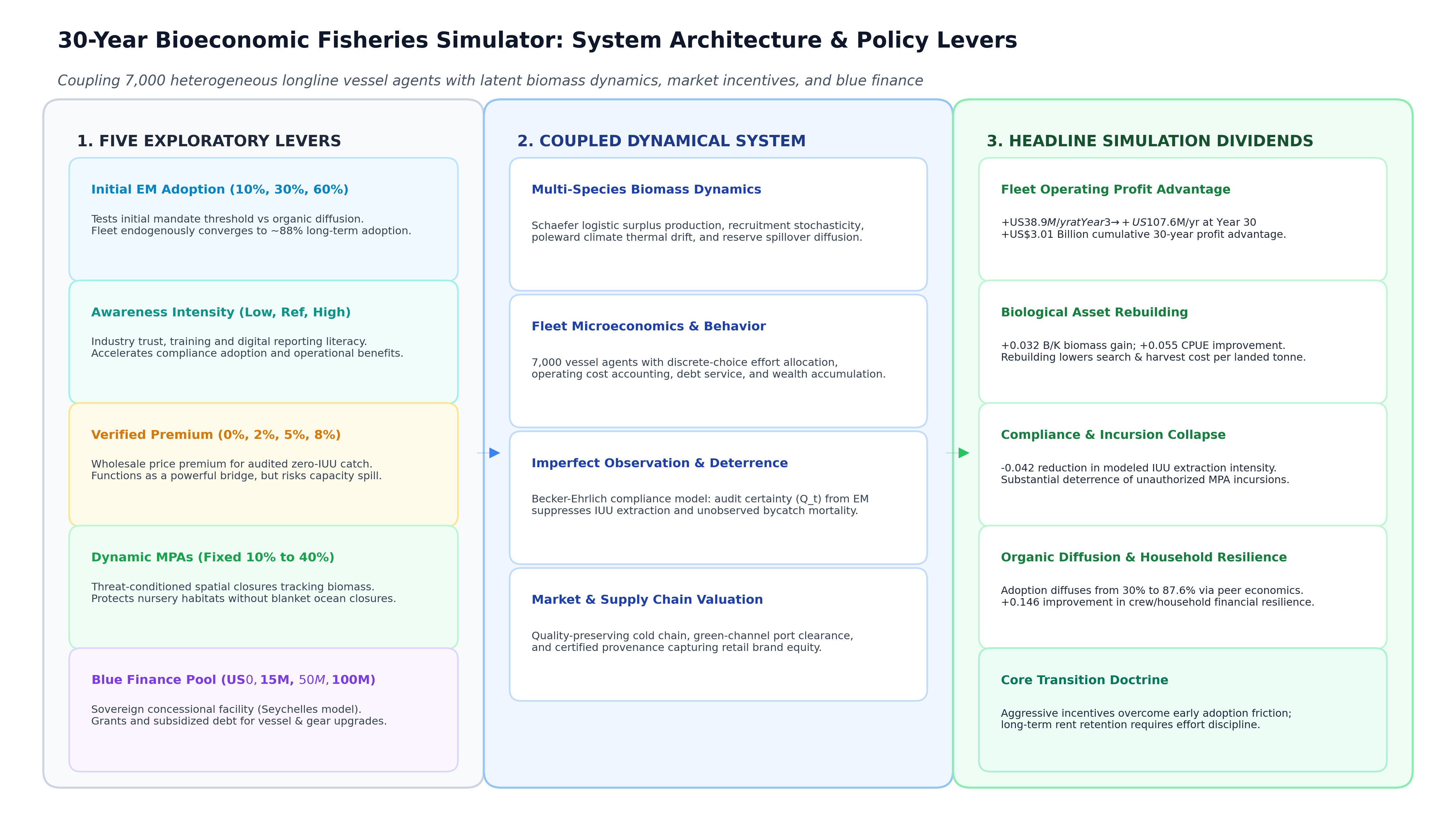
- Coupled bioeconomic methods: Below the narrative, we document the formal dynamical model coupling 7,000 heterogeneous vessels across multi-species Schaefer surplus production, Becker-Ehrlich deterrence, RUM effort choice, dynamic MPAs, and sovereign blue finance across 14 policy scenarios.
What a 30-year longline simulation
Electronic monitoring (EM) in fisheries is usually introduced through the language of compliance: cameras, sensors, electronic logbooks, traceability, observer substitution, reporting and enforcement. From the fisher’s point of view, the proposition can sound simple: install hardware, accept more scrutiny, create more data, and carry an additional operating burden so that someone else can regulate the fishery better. In this article, we ask can monitoring be designed so that the fisher is financially and operationally better off in the short term, while the fishery itself becomes more productive in the long term?
To explore that question, we built a stochastic 30-year Monte Carlo simulator representing a tuna-longline fleet with 7,000 vessel/operator agents. The model couples fish biomass, recruitment, fishing effort, catch, IUU behaviour, awareness, EM adoption, market prices, verified-catch premiums, marine protected area (MPA) policy, operating costs, vessel wealth, and blue finance.
We then ran a structured scenario sweep varying five levers: initial EM adoption, awareness intensity, verified-catch premium, MPA policy, and blue-finance availability. The purpose was not to create a forecast. The model is still an exploratory policy simulator whose biological, behavioural and financial coefficients must ultimately be calibrated against RFMO stock assessments, GFW effort data, observer/EM data, vessel economics and actual finance programmes. The useful question at this stage is not “what exactly will profit be in 2056?” It is which mechanisms consistently improve the economics of fishing, and which apparently attractive interventions create unintended effects? The results suggest a much stronger way to think about EM not as surveillance infrastructure, but as economic information infrastructure for a better-managed fishing asset.
The starting economic problem is bigger than the cost of a camera
The World Bank’s Sunken Billions Revisited estimated that poor fisheries management and depleted stocks cost global marine fisheries roughly US$83 billion in foregone annual economic benefits (World Bank, 2017). The core lesson is not simply that fish stocks need protection, it is that a degraded fishery is an inefficient economic asset: more vessels, fuel, labour and time can be required to produce less economic rent (Gordon, 1954; Schaefer, 1954; FAO, 1995). If monitoring only increases compliance cost, fishers may rationally resist it, but if monitoring helps move a fishery toward higher catch per unit effort (CPUE), lower uncertainty, lower illegal extraction, better quality realization, better market access and cheaper finance, then the economics look very different.
This is particularly important because the global market does not imply unlimited catch growth. OECD-FAO currently projects global demand for aquatic animal foods to grow about 12% over the next decade, while capture fisheries production grows only around 3.4% (OECD/FAO, 2024, 2025). It also projects real capture-fish prices to decline, in other words, the long-term opportunity is not simply “catch more and sell at a higher price.” It is to generate more economic value per unit of biological resource and per unit of fishing effort.
That is the economic target used in the simulation.
What is actually simulated?
The model contains a latent ecological, economic system and several imperfect observation channels, fish biomass evolves through stock growth, catch and environmental shocks. Fisher effort responds to profitability but is bounded to prevent unlimited expansion, awareness and trust influence EM adoption. Monitoring raises the probability that illegal activity is detected and reduces unreported fishing.
Importantly, Global Fishing Watch data would enter such a model as an observation of apparent fishing activity, not as exact ground truth. GFW itself cautions that AIS based apparent fishing activity can include searching and gear preparation and can contain false positives, gaps and vessel-classification errors (Global Fishing Watch, 2024a, 2024b). The model therefore treats AIS/GFW, logbooks, observers and EM as different observation channels around a latent real fishery.
EM can improve the observation quality because it provides vessel level evidence of catch and operations. NOAA’s Hawaiʻi longline pre-implementation evaluation found that EM review detected 98% of retained fish recorded by observers in the shallow set fishery and 100% in the deep set fishery, while review time for similar data collection could be substantially lower (Carnes et al., 2019). The simulator therefore does not assume that installing a camera magically creates fish. It changes information quality, incentives and behaviour, which inturn affect biomass, CPUE, costs and revenue over time.
The reference scenario
The reference intervention begins with 30% EM adoption, a moderate awareness campaign, a maximum 5% verified-catch premium, dynamic MPA management starting from 10%, and a US$15 million blue-finance pool. Each scenario was simulated over 30 years using paired stochastic worlds so that business as usual (BAU) and intervention runs experienced the same underlying environmental and market shocks.
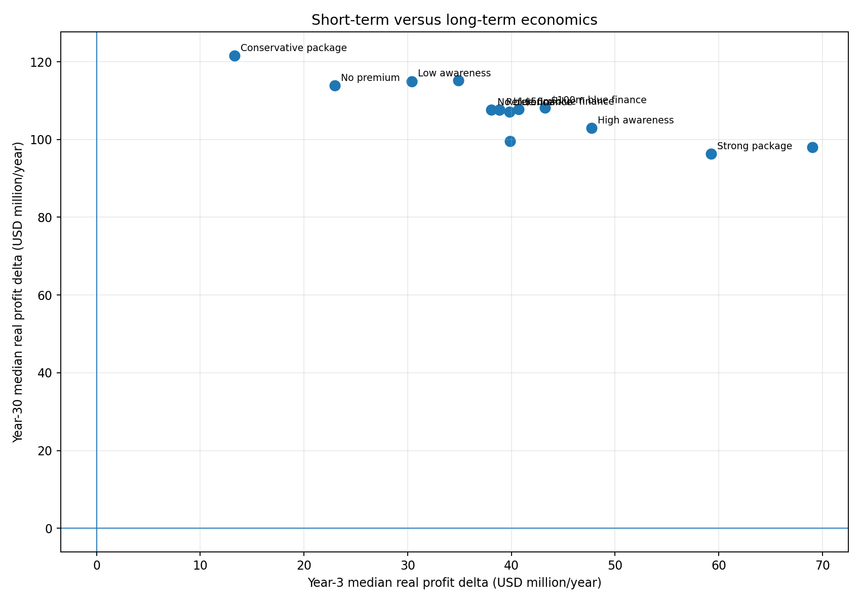
In the exploratory sweep, the reference intervention produced a median year-3 fleet profit advantage of approximately US$38.9 million per year relative to BAU. By year 30, the median annual advantage was approximately US$107.6 million, while cumulative real fleet profit over the 30 year horizon was about US$3.01 billion higher than BAU.
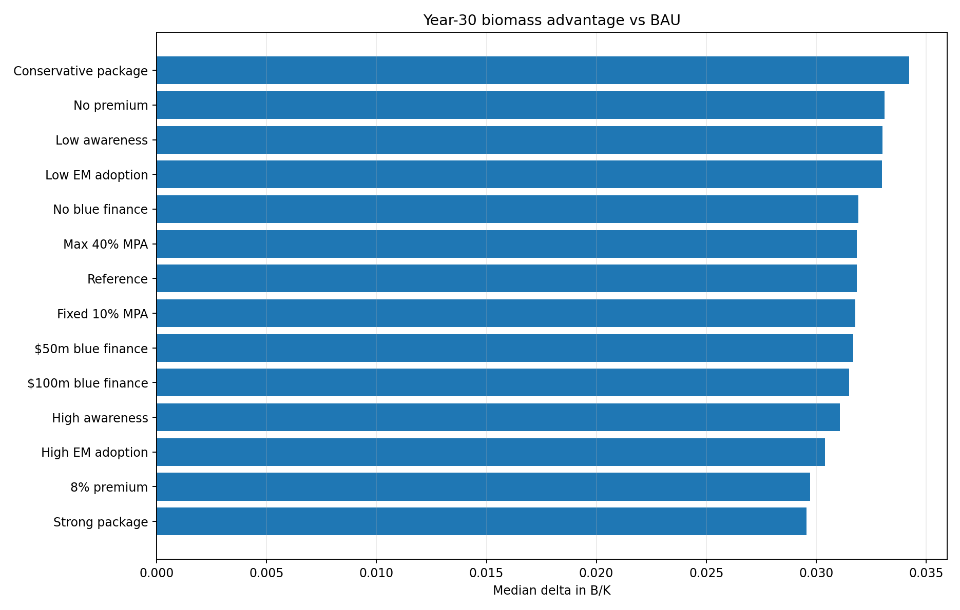
At the same time, the median biomass advantage reached roughly +0.032 in B/K, the CPUE index improved by approximately 0.055, and modeled IUU intensity fell by about 0.042 relative to BAU. Median EM adoption reached approximately 87.6% because adoption was allowed to diffuse through awareness, peer effects, observed benefits, trust and regulatory pressure rather than remaining fixed at the initial 30%.
These numbers should be interpreted as scenario outputs, not forecasts. What matters more is the structure of the result: short-term economics become positive before the ecological gain becomes large, while long-term economic advantage increasingly shifts toward resource productivity.
Awareness helps early, but awareness alone is not the long-term economic engine
We varied awareness intensity while keeping the broader intervention structure similar.
A low-awareness scenario produced a median year-3 profit advantage of about US$30.4 million. A high-awareness scenario increased this to roughly US$47.7 million. The mechanism is straightforward: greater awareness and trust accelerate adoption and behavioural change, so reporting, operational and compliance benefits appear sooner.
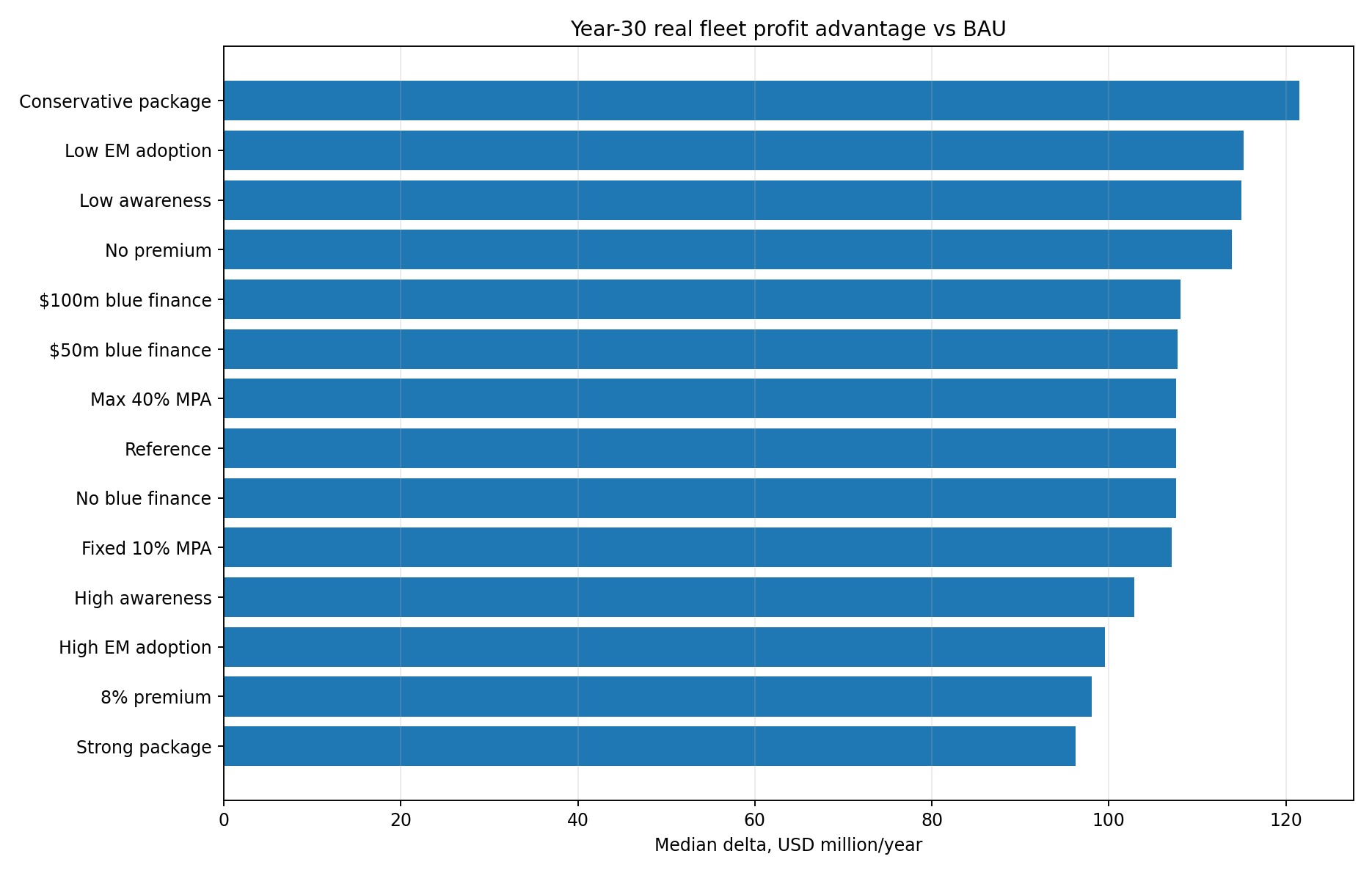
But an interesting reversal appears later. At year 30, the low-awareness case showed a profit advantage of about US$115.0 million, compared with about US$102.9 million under high awareness. Higher awareness was therefore clearly useful for the transition, but it was not automatically the long-term state.
Why? Because adoption and early economic benefits can also increase effort. If every gain from a more productive fishery is reinvested in additional hooks, trips and capacity, economic rent is partially dissipated. This is exactly why fisheries economics cannot be reduced to “more adoption is always better.”
The practical implication is important: awareness programmes should be paired with effort discipline and productivity objectives. The goal is not simply to maximize technology uptake, it is to move the fleet toward higher value per unit effort.
Initial EM adoption matters < system that follows it
We tested initial EM adoption at 10%, 30% and 60%.
The surprising result was that all three scenarios converged to roughly 87-88% adoption over the long run. A higher starting adoption rate improved early visibility and cumulative value, but the final adoption rate was driven much more by endogenous economics, peer effects and trust than by the starting percentage.
The 10% initial adoption case produced around US$34.9 million of year-3 profit advantage, while the 60% case produced about US$39.9 million. The difference is meaningful but not transformative. By year 30, the lower initial adoption case actually showed a slightly larger annual profit advantage than the high adoption case, although the high adoption case accumulated more total benefit over the full transition. The lesson is useful for implementation: a jurisdiction does not necessarily need to force the entire fleet into EM on day one. A credible first cohort can create the evidence and economic signal needed for diffusion, provided the rest of the system rewards verified fishing.
A premium helps adoption
One of the clearest findings came from varying the verified-catch premium.
With no premium at all, the model still produced a median year-3 profit advantage of approximately US$23.0 million and a year-30 advantage of approximately US$113.9 million. This is important because it means the long-run economic case does not depend on convincing consumers to pay a permanent sustainability premium.
At the other extreme, an 8% maximum premium produced approximately US$69.0 million of year-3 profit advantage far above the reference case. That makes a premium a powerful transition instrument. Yet the same scenario produced a lower year-30 annual profit advantage, about US$98.0 million, and a slightly smaller biomass and CPUE advantage.
The explanation is a fisheries economics feedback, higher early prices increase expected returns, which can increase fishing effort. If capacity growth is not managed, part of the premium is converted into additional effort rather than retained as fisher rent.
So the better policy is not “offer the largest possible premium forever.” It is: Use premiums, buyer guarantees and transition incentives to make adoption attractive in years 1-5; then allow the long-term value proposition to migrate toward lower cost per tonne, higher CPUE, market access, finance and risk reduction.
That is a much more resilient business model.
The resource effect influences long-term economics
The most important ecological pathway is not that monitoring creates more fish directly. It is that monitoring and awareness reduce the rate at which biological value is unnecessarily removed.
The model links EM and awareness to three mechanisms: lower unreported/IUU mortality, lower avoidable juvenile/bycatch mortality, and a stronger biomass sensitive effort response among monitored vessels. As these effects accumulate, biomass degradation slows, the fleet then fishes against a more productive stock.
The chain is:
Monitoring → better information and deterrence → lower hidden mortality → more biomass retained → stronger recruitment and availability → higher CPUE → less effort required per tonne → lower operating cost → higher economic rent.
This is a much stronger fisher proposition than “fish less today so that somebody may benefit in twenty years.” In the model, the fisher eventually benefits because the biological asset they depend on remains more productive.
The World Bank’s fisheries work points in the same direction at a global scale: depleted stocks and excess fishing effort dissipate economic rents, while rebuilding can allow greater sustainable harvest and substantially higher profits (World Bank, 2017). The model simply makes that principle operational at vessel/fleet level.
MPAs are useful, but bigger is not automatically better
We also varied MPA policy, in this particular parameter regime, allowing the dynamic controller to expand to 40% produced almost no additional effect relative to the reference maximum of 30%. A fixed 10% MPA also produced results remarkably close to the reference case.
This is not evidence that MPAs do not matter, it means that in these simulations the ecological risk controller rarely needed to push protected area coverage beyond the lower range, because monitoring, declining IUU and biomass response were already stabilizing the system.
This is an important modeling result because it argues against a simplistic “more MPA equals more benefit” narrative. The value of an MPA depends on where it is, when it is applied, how effort is displaced, and how mobile tuna stocks respond. Dynamic spatial management can therefore be more economically efficient than expanding static closure percentages without regard to risk.
For implementation, the implication is that EM can make MPA policy more targeted. Better spatial evidence allows authorities to protect high-risk periods or areas without unnecessarily removing fishing opportunity everywhere.
Blue finance changes who can afford the transition
The blue-finance scenarios produced a different type of benefit. Blue finance did not materially change biomass by itself. Instead, it affected the financial burden of making the transition.
The simulator follows the structure seen in the Seychelles blue-bond experience rather than assuming that an individual fisher issues a bond. A sovereign or institutional blue-finance pool is created centrally and then deployed through grants and concessional loans. The World Bank-supported Seychelles blue bond raised US$15 million, with proceeds supporting grants and investment for sustainable fisheries and ocean management; World Bank documentation describes US$3 million channelled through a grant mechanism and US$12 million through subsidized lending (World Bank Treasury, 2025).
The Development Bank of Seychelles currently describes its Blue Investment Fund as offering eligible sustainable-fisheries loans from US$10,000 to US$3 million at 4% interest with repayment terms up to 15 years (Development Bank of Seychelles, 2025).
In our reference scenario, the US$15 million pool generated only a modest incremental fleet-wide economic effect because eligibility rules and annual disbursement constraints meant that only part of the capital reached vessel operators. That is exactly the sort of outcome a policy model should expose.
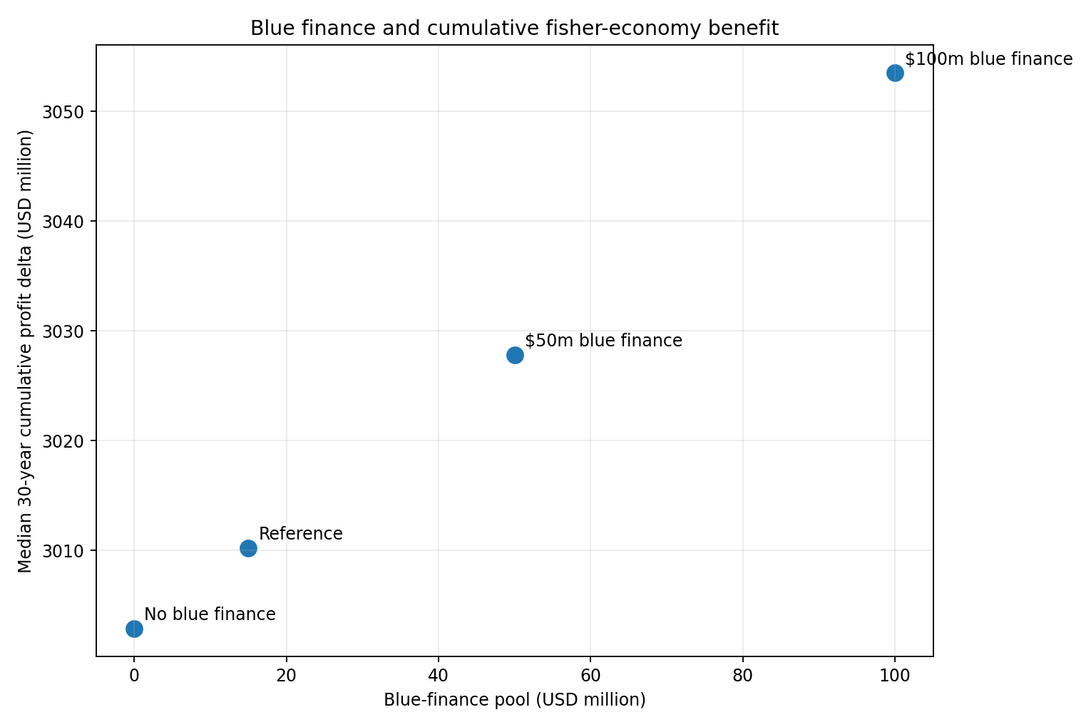
Removing blue finance reduced the 30-year cumulative profit advantage by roughly US$7 million relative to the reference case. Increasing the nominal pool to US$50 million raised the cumulative advantage by roughlyUS$25 million versus no blue finance, while a US$100 million pool increased it by roughly US$51 million. Year-3 profit advantage also rose progressively as the pool increased.
However, the simulations show that capital size alone is not enough, a US$100 million fund did not deploy US$100 million to fishers. Eligibility, trust, compliance history, loan limits and the number of finance ready projects constrained deployment. This is realistic, blue finance only changes livelihoods if fishers can actually access it.
The mechanism becomes compelling when finance is linked to useful investments rather than used as a generic reward:
Verified fishing history → eligibility → cheaper refinancing and productive capex → lower debt service + fuel/quality upgrades → higher cash-flow resilience.
That can improve a fisher’s lifestyle in ways that a sustainability label alone cannot: lower financing stress, lower annual debt burden, more reliable equipment, safer operations, improved cold chain, and greater resilience when catch or prices fluctuate.
The biggest lesson: the strongest short-term package is not necessarily the best long-term package
We compared two combined interventions.
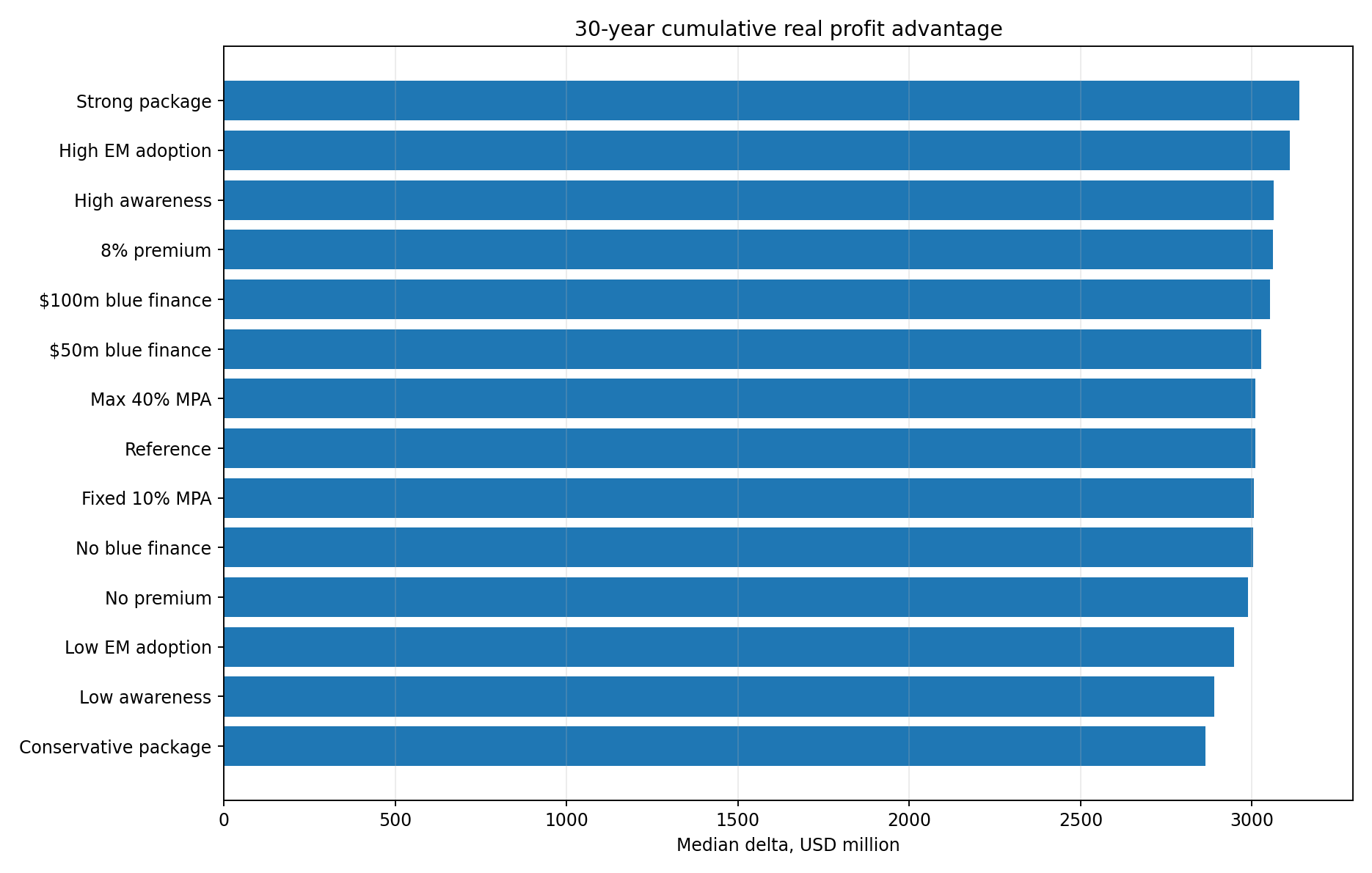
A “strong” package used 50% initial EM adoption, high awareness, a 5% premium, a larger premium market, a 30% MPA ceiling and US$50 million of blue finance. It generated a US$59.3 million median year-3 profit advantage and the highest cumulative benefit among the combined packages, about US$3.14 billion over 30 years.
A more conservative package used 20% initial adoption, weaker awareness, a 2% premium, a 20% MPA ceiling and US$15 million of blue finance. It generated only about US$13.3 million of year-3 advantage, but by year 30 its annual profit advantage was approximately US$121.5 million, the highest among the tested scenarios. It also produced the largest biomass and CPUE advantages in the sweep.
This is the central result of the exercise.
Aggressive incentives are excellent for overcoming the adoption barrier. Moderate long-term pressure is better for retaining the resource rent.
A sensible transition therefore looks staged:
Years 1-3: subsidize equipment, automate reporting, reduce inspection burden, create buyer/offtake incentives, use grants and cheap working capital.
Years 3-8: phase out blanket subsidies, reward verified performance, introduce insurance and credit differentiation, maintain targeted market incentives.
Years 8-30: let biomass, CPUE, lower cost per tonne, market access, trusted-vessel status and finance become the dominant economic benefits, while constraining excess capacity growth.
The objective is not to make the fisher permanently dependent on a subsidy. It is to finance the crossing from an unverified, high-uncertainty fishery to a verified, lower-risk, more productive fishery.
What does “better lifestyle” mean in this model?
It is easy to use “fisher wellbeing” too casually, the simulator therefore avoids claiming that cameras directly improve subjective quality of life. Instead it tracks economic proxies that can plausibly affect household and crew wellbeing: annual vessel income, debt-service burden, solvency, effort/days-at-sea burden and a transparent household-resilience index.
The reference intervention improves the resilience proxy by roughly 0.146 relative to BAU at year 30. The exact value is model specific, but the pathway is economically intuitive: higher income stability, lower debt pressure and higher CPUE can make a household less vulnerable to one poor trip, one fuel-price shock or one equipment failure.
This is where blue finance can be particularly valuable, a concessional loan used only to buy a monitoring system is not especially transformative. A finance facility that uses verified fishing data to refinance expensive debt, improve fuel efficiency, upgrade refrigeration, fund safer gear or provide working capital can materially change the vessel’s economics.
In that model, monitoring data becomes credit infrastructure.
EM also changes the value of information itself
There is another benefit that is often missed. Fisheries management operates under uncertainty. Authorities do not observe the true stock, true fishing effort or true IUU activity directly. They infer them from logbooks, observers, AIS/VMS, surveys and models.
Electronic monitoring changes the observation system. That improves not only compliance enforcement but also stock assessment, risk-based inspection, MPA targeting and market verification.
This distinction matters because Global Fishing Watch’s AIS-based activity is enormously useful for large-scale spatial context, but GFW explicitly describes it as apparent fishing activity (Global Fishing Watch, 2024a, 2024b). EM can complement that signal with onboard evidence of what was actually caught and handled.
Better information can therefore reduce the cost of bad management decisions. That economic value is partly public better science and governance but it can flow back to fishers through more stable quotas, fewer unnecessary inspections, less blanket regulation and more targeted management.
The simulation also shows what will not work
The scenarios provide several warnings.
A compliance-only deployment is weak because costs arrive before benefits. A permanent premium is fragile because premium demand can saturate and higher prices can stimulate excess effort. A huge blue-finance pool is ineffective if fishers cannot meet eligibility requirements or projects are not investment-ready. More MPA coverage is not automatically more efficient if the protected area is not aligned with ecological risk. And maximizing adoption without managing fishing capacity can simply convert productivity gains into additional effort.
The economic proposition therefore has to be designed as a system.
EM should automate reporting rather than add paperwork. Monitoring should reduce inspection friction for trusted vessels. Verified data should improve market access. Finance should reward verified performance but also fund productive upgrades. Awareness should explain the benefits, not merely the rules. Management should retain enough of the biomass gain that CPUE increases rather than allowing every gain to be dissipated through more effort.
So, does EM improve fisher livelihoods?
The honest answer is not “a camera always makes a fisher richer.” That would be an indefensible claim. The stronger conclusion from the simulations is this:
When EM is deployed as part of an economic transition combining reporting automation, lower regulatory friction, improved market access, temporary premiums, better management, targeted blue finance and disciplined effort; it can make verified fishing economically preferable to unverified fishing in the short term while preserving a more productive fishery in the long term.
The Eastern Pacific tuna EM cost benefit work provides an external point of comparison: an analysis highlighted by Pew estimated that broader EM could produce substantial net benefits over ten years through improved science, bycatch mitigation, compliance and potential market benefits (Pew Charitable Trusts, 2020). That does not prove the parameters used in our simulator, but it reinforces the central idea that EM’s value is broader than the hardware itself.
The policy objective should therefore change from: “How do we convince fishers to accept monitoring?” To: “How do we make verified fishing the better business model?”
If the answer includes lower operational friction today, better access to buyers and finance tomorrow, and a more productive stock over the next decade, then monitoring stops looking like a compliance tax. It starts to look like infrastructure for the economic modernization of the fishery.
Technical Methodology & Model Definitions
This technical section documents the mathematical and computational framework underpinning the 30-year tuna-longline Monte Carlo experiments. The implementation operates as an integrated policy operating model:
\[X_{t+1} = F(X_t, U_t, \theta, \varepsilon_t)\]where \(X_t\) is the latent multi-dimensional state vector of the fishery, fleet, and markets; \(U_t\) is the policy control vector (EM subsidies, verified price premiums, MPA boundaries, concessional blue finance pools); \(\theta\) is the parameter set governing biological surplus production, cost structures, and behavioral response; and \(\varepsilon_t\) represents stochastic environmental, recruitment, climate, and macroeconomic price innovations.
The simulator deliberately separates four distinct sources of variation:
- Parameter uncertainty: Intrinsic growth rates (\(r_s\)), carrying capacities (\(K_s\)), baseline catchabilities (\(q_s\)).
- Process stochasticity: Annual recruitment deviations, sea-surface temperature anomalies, and global commodity price innovations.
- Agent heterogeneity: Vessel-specific catchability multipliers, engine fuel efficiencies, operator debt profiles, initial regulatory trust, administrative burden, and product-quality skill.
- Policy hypotheses: Subsidy rates, verified export premium ceilings, concessional loan availability, and spatial closure regimes.
1. Simulation Domain & Fleet Specifications
- Fleet scale: \(N_v = 7{,}000\) heterogeneous longline vessels and operators.
- Agent heterogeneity attributes:
- Relative catchability multiplier: \(q^{rel}_i \sim \operatorname{Lognormal}(0, 0.22)\)
- Fuel consumption efficiency: \(\eta^{fuel}_i \sim \operatorname{Uniform}(0.85, 1.15)\)
- Regulatory trust baseline: \(Trust_{i,0} \sim \operatorname{Beta}(2.5, 4.0)\)
- Operator debt load: \(Debt_{i,0} \sim \operatorname{Uniform}(\$40{,}000, \$180{,}000)\)
- Administrative compliance burden: $AdminBurden_i \sim \operatorname{Uniform}(0.8, 1.3)$
- Quality handling skill: \(QualitySkill_i \sim \operatorname{Uniform}(0.0, 1.0)\)
- Species groups: Three major pelagic tuna stocks: Yellowfin tuna (Thunnus albacares, YFT), Bigeye tuna (Thunnus obesus, BET), and Albacore tuna (Thunnus alalunga, ALB), each modeled with distinct intrinsic growth rates, carrying capacities, catchabilities, and ex-vessel prices.
- Temporal horizon: 30 years updated at annual discrete time-steps, with internal sub-step accounting for seasonal effort allocation, debt service, and capital amortization.
2. Multi-Species Biological Dynamics
The ecological foundation builds on species-specific surplus production in the Gordon-Schaefer family (Schaefer, 1954; FAO, 1995, 2004):
\[P_{s,t} = r_s B_{s,t} \left(1 - \frac{B_{s,t}}{K_s}\right)\]where \(B_{s,t}\) is stock biomass, \(r_s\) is intrinsic biological growth, and \(K_s\) is regional carrying capacity. To account for climate variability and marine heatwaves, annual recruitment incorporates multiplicative environmental and climate shocks:
\[P^*_{s,t} = P_{s,t} \exp\left(0.35 \, \epsilon^{climate}_t + \epsilon^{recruit}_{s,t}\right)\]Under policy interventions, effective reproductive productivity benefits from a bounded protection factor:
\[P^{I}_{s,t} = P^*_{s,t} \left(1 + \rho_R \cdot Protection_t\right), \quad \text{where } Protection_t = \operatorname{clip}(A_t Z_t T_t, \, 0, \, 1)\]Here, \(A_t\) is the fleet EM adoption rate, \(Z_t\) is average fleet awareness/literacy, \(T_t\) is regulatory trust, and \(\rho_R\) is the maximum recruitment preservation coefficient. This is an explicit policy hypothesis: cameras do not spawn fish; rather, continuous monitoring eliminates hidden discard mortality and protects juvenile aggregations, directly boosting effective recruitment.
3. Harvest and Latent Mortality Accounting
Total fishing mortality is partitioned into legal retained catch and two latent mortality channels:
- Legal Catch Equation: Following standard Gordon-Schaefer formulations (Schaefer, 1954; FAO, 2005): \(H_{s,t} = q_s E^{eff}_t B_{s,t}, \quad \text{subject to } H_{s,t} \le 0.18 B_{s,t}\)
- Illegal, Unreported, and Unregulated (IUU) Mortality: \(M^{IUU}_t = 0.60 \, I_t H_t\) where \(I_t \in [0, 1]\) represents the latent fleet-wide IUU poaching intensity index.
- Avoidable Bycatch and Discard Mortality: Under Business-as-Usual (BAU), avoidable mortality expands with poaching: \(M^{avoid, BAU}_t = H_t m_0 (1 + 0.15 I_t)\) Under EM intervention, verifiable deployment of mitigation gear (circle hooks, tori lines) suppresses discard mortality as fleet adoption and awareness grow (Gilman et al., 2014; van Helmond et al., 2020): \(m_t = m_0 (1 - \rho_M Protection_t) \implies M^{avoid, INT}_t = H_t m_t\)
The comprehensive biological stock transition for each species is:
\[B_{s,t+1} = B_{s,t} + P_{s,t} - H_{s,t} - M^{IUU}_{s,t} - M^{avoid}_{s,t}\]Hidden mortalities are partitioned across species proportional to their catch share. This structural coupling establishes the core biological transmission channel:
\[EM \, (A_t) \uparrow, \; Awareness \, (Z_t) \uparrow \implies IUU \, (I_t) \downarrow, \; M^{avoid} \downarrow \implies B_{s,t+1} \uparrow \implies CPUE \uparrow\]4. Fleet Effort Allocation, CPUE, and Bounded Profit Response
Fleet raw nominal effort aggregates vessel-specific effort scaled by relative individual catchability:
\[E_t = \sum_{i=1}^{N_v} e_{i,t} q^{rel}_i\]Effective effort \(E^{eff}_t\) accounts for spatial MPA closure access and voluntary conservation responses under biomass scarcity:
\[Access_t = 1 - 0.70 M_t\] \[Scarcity_t = \operatorname{clip}\left(\frac{0.62 - B_t/K}{0.22}, \, 0, \, 1\right)\] \[ConservationResponse_t = 1 - 0.18 A_t Z_t Scarcity_t\] \[E^{eff}_t = E_t \cdot Access_t \cdot ConservationResponse_t\]Catch-Per-Unit-Effort is evaluated as:
\[CPUE_t = \frac{H_t}{E_t}\]Bounded Gordon-Schaefer Effort Response
In an open-access fishery, positive economic rents attract capital and effort until rents are fully dissipated (Gordon, 1954). The simulator incorporates profit-responsive effort dynamics but bounds expansion to reflect licensing, capital constraints, and vessel physical limits:
\[e_{i,t+1} = e_{i,t} \exp\left(\gamma_s Margin_{i,t} Room_{i,t}\right)\]where:
\[Margin_{i,t} = \operatorname{clip}\left(\frac{\Pi_{i,t}}{Cost_{i,t}}, \, -0.8, \, 1.2\right)\] \[Room_{i,t} = \operatorname{clip}\left(1 - \frac{e_{i,t}}{E^{cap}_s}, \, 0.05, \, 0.85\right)\]Under policy interventions, the fleet operates with a lower expansion coefficient \(\gamma_s\) and a tighter capacity cap \(E^{cap}_s\), reflecting managed-access conditions that prevent rebuilt stock wealth from being dissipated in excess capacity (World Bank, 2017).
5. Awareness Diffusion, Compliance Capital, and Logistic Adoption
Awareness Dynamics
Awareness \(Z_{i,t} \in [0, 1]\) evolves through public campaigns, peer observation, observed economic returns among adopters, and natural decay:
\[Z_{i,t+1} = Z_{i,t} + \alpha_C Campaign_t + \alpha_P Peer_t + \alpha_B Benefit_t T_{i,t} + \alpha_R Resource_t - \delta_Z Z_{i,t}\]where \(Campaign_t \in [0, 1]\) represents public regulatory outreach intensity, \(Peer_t = A_t\) is the prevailing fleet adoption fraction, \(Benefit_t = \max(0, Margin^{adopter}_t - Margin^{non}_t)\) is the observed profit advantage of adopters scaled by vessel trust \(T_{i,t}\), \(Resource_t \propto (0.62 - B_t/K)\) is the perceived stock scarcity signal, \(\delta_Z = 0.08\) is the annual awareness decay rate, and \(\alpha_C, \alpha_P, \alpha_B, \alpha_R\) are response sensitivity weights (\(0.25, 0.20, 0.15, 0.10\)).
Compliance Capital and Trust Formation
The simulator separates general regulatory trust from accumulated vessel-specific compliance capital:
\[VTrust_{i,t+1} = 0.90 VTrust_{i,t} + 0.12 A_{i,t} Z_{i,t} - Penalty_t\]where \(Penalty_t\) represents the trust deduction triggered by detected fishery infractions (\(\propto I_t\)). General trust slowly converges toward this verified history. Verified compliance capital unlocks tangible benefits: reduced dockside inspection frequency, priority port clearance, and eligibility for concessional finance.
Logistic Adoption with Churn
Adoption is stochastic and reversible. A latent adoption score combines awareness, peer adoption, trust, net economic benefits, regulatory pressure, and costs:
\[S_{i,t} = \beta_0 + \beta_Z Z_{i,t} + \beta_P Peer_t + \beta_T Trust_{i,t} + \beta_B Benefit_t + \beta_R RegPressure_t - \beta_C Cost_t\]where \(RegPressure_t\) reflects statutory enforcement expectations, \(Cost_t\) is annualized hardware and airtime expenditure, and \(\beta_0 \dots \beta_C\) are logistic utility coefficients. The adoption probability follows a logistic distribution (Bass, 1969):
\[\sigma(S_{i,t}) = \frac{1}{1 + e^{-S_{i,t}}}\]If verified price premiums or blue-finance benefits deteriorate, vessels face an endogenous churn probability, permitting reversible disadoption.
6. Becker-Ehrlich Latent IUU Deterrence Model
Non-compliance is modeled as an endogenous economic decision under imperfect enforcement (Becker, 1968; Charles et al., 1999; FAO, 2002).
Detection Probability
Under the intervention, detection probability expands with EM fleet coverage, statutory enforcement, and accumulated compliance history:
\[P^{detect}_t = \operatorname{clip}\left(0.12 + \delta_A A_t + 0.10 Enforcement + 0.08 Trusted_t, \, 0, \, 0.94\right)\]Latent IUU Behavioral Update
Poaching intensity \(I_t \in [0, 1]\) expands under resource scarcity and high fish prices, but contracts as detection probability and awareness rise:
\[I_{t+1} = I_t + \alpha_S Scarcity_t + \alpha_P PriceSignal_t - \beta_D P^{detect}_t I_t - \beta_Z Z_t I_t\]where \(PriceSignal_t = \operatorname{clip}((P_t - \bar{P}_0)/\bar{P}_0, 0, 1)\) captures the marginal economic incentive to poach when market prices surge above baseline \(\bar{P}_0\), \(\alpha_S, \alpha_P\) govern poaching escalation sensitivities (\(0.045, 0.035\)), and \(\beta_D, \beta_Z\) capture deterrence from detection and community awareness (\(0.180, 0.060\)). Under BAU, detection probability remains low (\(P^{detect} \le 0.12\)), allowing IUU poaching to persist as a rational response to stock depletion.
7. Dynamic Threat-Conditioned MPA Controller
The spatial policy controller adjusts closed-area coverage \(M_t \in [M_{min}, M_{max}]\) dynamically based on ecological risk versus governance relief:
\[Risk_t = \left(0.62 - \frac{B_t}{K}\right) + 0.70 (I_t - 0.06)\] \[Relief_t = 0.10 A_t Z_t\] \[\Delta M_t = \operatorname{clip}\left(0.045(Risk_t - Relief_t), \, -0.012, \, 0.028\right)\] \[M_{t+1} = \operatorname{clip}\left(M_t + \Delta M_t, \, M_{min}, \, M_{max}\right)\]When biomass falls or poaching spikes, the controller automatically expands MPA boundaries. When high EM adoption and awareness suppress illegal extraction, governance relief allows closures to relax toward \(M_{min}\), avoiding unnecessary loss of fishing grounds.
8. Observation Model: Latent Truth vs. Imperfect Channels
A critical architectural distinction is that regulatory authorities never directly observe true biomass, true fishing effort, or true IUU extraction. They observe noisy signals across distinct channels:
- AIS / Global Fishing Watch Telemetry: \(Y^{GFW}_t = H_{AIS}(E^{true}_t) + \epsilon^{AIS}_t\) As documented by GFW, AIS algorithms infer apparent fishing behavior, which includes searching, maneuvering, and gear deployment, subject to satellite reception gaps and intentional transponder disabling (Global Fishing Watch, 2024a, 2024b).
- Electronic Monitoring Optical/Sensor Stream: \(Y^{EM}_t = H_{EM}(Catch^{true}_t, Interactions_t) + \epsilon^{EM}_t\) NOAA Fisheries trials demonstrate 98–100% detection for retained target tuna, but lower accuracy for rare bycatch and discard release condition without secondary sensor gating (Carnes et al., 2019).
- Logbook Self-Reporting: \(Y^{log}_t = H_{log}(Catch^{true}_t, ReportingBehaviour_t) + \epsilon^{log}_t\) Historically biased by under-reporting of juvenile catch, discard avoidance, and quota gaming.
By explicitly distinguishing latent state variables from observation equations, the simulator captures how EM reduces administrative uncertainty.
9. Market Demand Frontier, Ex-Vessel Price Feedback, and Inflation
Growing Demand Frontier
Rather than assuming a static market capacity, global demand capacity expands according to FAO aquatic-food consumption projections (OECD/FAO, 2024, 2025):
\[D_{s,t+1} = D_{s,t} \exp\left(g_{D,s} + 0.20 \epsilon^{market}_{s,t}\right)\]with annual drift rates \(g_{D,YFT} = 1.2\%\), \(g_{D,BET} = 1.3\%\), and \(g_{D,ALB} = 1.0\%\).
Endogenous Ex-Vessel Price Feedback
The fleet’s harvest interacts with global demand through an endogenous supply-gap signal:
\[G_{s,t} = \ln\left(\frac{D_{s,t}}{H_{s,t}}\right)\] \[g^P_{s,t} = 0.70 \mu_{P,s} + 0.025 G_{s,t} + \epsilon^{market}_{s,t}\] \[P_{s,t+1} = P_{s,t} \exp(g^P_{s,t})\]Excess supply depresses ex-vessel price growth, while supply deficits support prices.
Real vs. Nominal CPI Inflation
A separate consumer price index tracks general inflation (\(CPI_{t+1} = CPI_t e^{\pi}\)), ensuring that all 30-year welfare metrics reflect real economic rent rather than nominal inflation artifacts.
10. Verified Premium and Market-Access Capacity
A statutory price premium \(\rho_t\) does not automatically apply to an unlimited volume of catch. Verified demand is capacity-constrained:
\[C^{premium}_t = \operatorname{clip}(C_0 + 0.10 Trusted_t, \, 0.15, \, 0.70)\] \[Coverage_t = \min(A_t, \, C^{premium}_t)\]The realized premium per adopting vessel is:
\[\rho^{real}_t = \rho_t \frac{Coverage_t}{A_t}\]When EM adoption outpaces high-end certified seafood demand, the realized premium naturally dilutes. This mechanism prevents the model from relying on permanent consumer price subsidies.
11. Microeconomic Benefit Stack Formulation
For each vessel \(i\) in year \(t\):
\[Revenue_{i,t} = BaseCatchRevenue + Premium + QualityGain + MarketAccessValue + PaymentSpeedValue\] \[Cost_{i,t} = BaseOperatingCost + FinanceCost + EMCost - \sum \text{Savings}\]The six tangible microeconomic channels comprise:
- Reporting savings (\(S^{report}_{i,t}\)): Automated e-logbook population and automated sensor reporting reduce captain and crew paperwork (\(S^{max}_{report} = 0.025\), capping savings at 2.5% of baseline operating expenditure): \(S^{report}_{i,t} = Cost^{base}_{i,t} A_{i,t} \min(S^{max}_{report}, \, 0.010 + 0.009 Z_{i,t}) \times AdminBurden_i\)
- Inspection savings (\(S^{inspect}_{i,t}\)): Trusted-vessel status shifts vessels to low-friction, risk-stratified dockside audits (\(S^{max}_{inspect} = 0.018\), capping savings at 1.8% of operating costs): \(S^{inspect}_{i,t} = Cost^{base}_{i,t} A_{i,t} \min(S^{max}_{inspect}, \, 0.004 + 0.010 Trust_{i,t})\)
- Operational efficiency (\(S^{oper}_{i,t}\)): Fuel optimization analytics, haul timing, and handling telemetry (\(S^{max}_{oper} = 0.040\), capping savings at 4.0% of operating costs), where \(Maturity_t = \operatorname{clip}((t-2)/6, 0, 1)\) reflects the learning curve required to master onboard analytics: \(S^{oper}_{i,t} = Cost^{base}_{i,t} A_{i,t} \min(S^{max}_{oper}, \, 0.008 + 0.030 Z_{i,t} Maturity_t)\)
- Quality realization gain (\(QGain_{i,t}\)): Onboard cold-chain sensor monitoring and verified handling preserve sashimi-grade quality (\(q_{max} = 0.035\), allowing up to a 3.5% revenue uplift), supplemented by capex upgrades \(CapexQuality_i\): \(QGain_{i,t} = Revenue^{base}_{i,t} A_{i,t} \left[(0.007 + q_{max} QualitySkill_i) Z_{i,t} + CapexQuality_i\right]\)
- Market access insurance (\(MValue_{i,t}\)): Traceability protects access to stringent import markets (US SIMP, EU IUU Regulation) even in the absence of a price premium (\(m_{max} = 0.020\), representing a 2.0% protected revenue share), where \(VerifiedAccess_t\) is the compliance-verified trade channel access fraction: \(MValue_{i,t} = Revenue^{base}_{i,t} A_{i,t} (0.006 + m_{max} Trusted_i) VerifiedAccess_t\)
- Payment settlement speed (\(PValue_{i,t}\)): Accelerated invoice factoring and working capital savings from trusted digital landing manifests (\(p_{max} = 0.010\), saving up to 1.0% in working capital financing costs): \(PValue_{i,t} = Revenue^{base}_{i,t} A_{i,t} (0.0025 + p_{max} Trusted_i)\)
12. Sovereign Blue Finance Mechanism (Seychelles Model)
The blue-finance facility reflects sovereign debt structures rather than individual vessel bond issuance (World Bank Treasury, 2025; Development Bank of Seychelles, 2025):
\[\text{Sovereign Blue Bond} \longrightarrow \text{Central Pool} \longrightarrow \text{Grants } (\lambda_G) + \text{Concessional Loans } (\lambda_L) \longrightarrow \text{Eligible Fleet}\]Eligibility Scoring
Vessels qualify for concessional financing based on compliance capital and low IUU history:
\[C_{i,t} = \operatorname{clip}(0.55 + 0.40 Trusted_{i,t} - 0.30 I_t, \, 0, \, 1) \ge \tau_C, \quad \text{with } A_{i,t} = 1 \text{ and } Trust_{i,t} \ge \tau_T\]Debt Refinancing Channel
A fraction \(\lambda_R\) of concessional credit replaces high-cost commercial debt:
\[Refinance_{i,t} = \lambda_R Loan_{i,t} \implies Saving^{interest}_{i,t} = BlueDebt_{i,t} (r_{market} - r_{blue})\]where market interest rates are modeled at 8.5% and concessional blue-finance rates at 4.0% (Development Bank of Seychelles, 2025).
Productive Capex Channel
The remaining loan portion \(\lambda_C Loan_{i,t}\) finances productive equipment upgrades:
\[Upgrade_{i,t+1} = \operatorname{clip}\left(Upgrade_{i,t} + \frac{Capex_{i,t}}{\$60{,}000}, \, 0, \, 1\right)\]which lowers vessel unit operating costs and enhances fish cold-chain preservation.
13. Fisher Household Resilience Model
To avoid vague wellbeing claims, the model tracks concrete economic proxies:
- Debt-Service Ratio (DSR): \(DSR_{i,t} = \frac{AnnualDebtService_{i,t}}{Revenue_{i,t}}\)
- Days-at-Sea / Effort Burden Index: \(DaysAtSeaIndex_t \propto \frac{MeanEffort_t}{CPUE_t}\)
- Household Resilience Index: \(Resilience_t = 0.45 \, IncomeComponent_t + 0.30 \, DebtComponent_t + 0.25 \, EffortComponent_t\)
Resilience improves when vessel net income rises, debt-service obligations contract, and higher CPUE reduces the days at sea required to meet harvest targets.
14. Coupled System Feedback Structure (The 7 Feedback Loops)
The emergent behavior of the simulator is driven by seven coupled bioeconomic feedback loops:
- Ecological-Economic Feedback: Biomass \(\rightarrow\) Catch \(\rightarrow\) Revenue \(\rightarrow\) Profit \(\rightarrow\) Effort Reinvestment \(\rightarrow\) Future Biomass.
- Monitoring-Compliance-Resource Feedback: EM \(\rightarrow\) Detection Probability \(\uparrow \rightarrow\) IUU Poaching \(\downarrow \rightarrow\) Hidden Discard Mortality \(\downarrow \rightarrow\) Stock Biomass \(\uparrow \rightarrow\) CPUE \(\uparrow\).
- Awareness-Adoption-Peer Feedback: Awareness Campaign \(\rightarrow\) First Adopters \(\rightarrow\) Observed Microeconomic Savings \(\rightarrow\) Peer Imitation \(\rightarrow\) Accelerated Diffusion.
- Market Supply-Gap Feedback: Total Landings \(\leftrightarrow\) Growing Global Demand \(\rightarrow\) Price Adjustment \(\rightarrow\) Revenue \(\rightarrow\) Profit \(\rightarrow\) Fleet Effort.
- Verified Premium Saturation Feedback: Fleet Adoption \(\uparrow \rightarrow\) Verified Landings \(\uparrow \rightarrow\) Premium Market Capacity Exceeded \(\rightarrow\) Realized Premium Dilution.
- Blue Finance Credit Feedback: Verified Compliance History \(\rightarrow\) Concessional Loan Eligibility \(\rightarrow\) Debt Refinancing + Capex Upgrades \(\rightarrow\) Lower Debt Service + Lower Fuel Cost \(\rightarrow\) Enhanced Vessel Solvency.
- Risk-Threat Governance Feedback: Stock Depletion / High IUU \(\rightarrow\) Threat Controller Expands MPA \(\rightarrow\) Effective Effort Restricted \(\rightarrow\) Stock Rebuilding \(\rightarrow\) Governance Relief Allows Spatial Re-opening.
15. The 14 Policy Scenarios & Comparative Analysis
The simulation evaluated fourteen structured policy packages across 24 paired Monte Carlo replicates, testing variations in initial EM coverage, awareness campaigns, price premiums, MPA ceilings, and blue-finance pools:
| Scenario Label | Initial EM (\(A_0\)) | Awareness Intensity | Price Premium (\(\rho^{max}\)) | MPA Closure Regime | Blue Finance Pool |
|---|---|---|---|---|---|
| Reference | 30% | Moderate | 5% max | Dynamic (10%–30%) | US$15M |
| Conservative package | 20% | Low | 2% max | Dynamic (10%–20%) | US$15M |
| Strong package | 50% | High | 5% max (wide market) | Dynamic (10%-30%) | US$50M |
| Low EM adoption | 10% | Moderate | 5% max | Dynamic (10%–30%) | US$15M |
| High EM adoption | 60% | Moderate | 5% max | Dynamic (10%–30%) | US$15M |
| Low awareness | 30% | Low | 5% max | Dynamic (10%–30%) | US$15M |
| High awareness | 30% | High | 5% max | Dynamic (10%–30%) | US$15M |
| No premium | 30% | Moderate | 0% | Dynamic (10%–30%) | US$15M |
| 8% premium | 30% | Moderate | 8% max | Dynamic (10%–30%) | US$15M |
| Fixed 10% MPA | 30% | Moderate | 5% max | Static 10% | US$15M |
| Max 40% MPA | 30% | Moderate | 5% max | Dynamic (10%–40%) | US$15M |
| No blue finance | 30% | Moderate | 5% max | Dynamic (10%–30%) | US$0M |
| $50m blue finance | 30% | Moderate | 5% max | Dynamic (10%–30%) | US$50M |
| $100m blue finance | 30% | Moderate | 5% max | Dynamic (10%–30%) | US$100M |
Deconstruction of Key Findings Across Scenarios
- The Short-Term Sprint vs. Long-Term Rent Frontier (Figures 2, 3, & 6):
- The Strong package generates high early returns (+US$59.3M/yr at Year 3) and the largest 30-year cumulative undiscounted profit (+US$3.14B). However, by Year 30, its annual profit advantage ranks lowest among interventions (+US$96.1M/yr) because strong early profits stimulate excess effort reinvestment, partially dissipating the biological rent.
- The Conservative package generates modest early cash flows (+US$13.3M/yr at Year 3), but ranks #1 in terminal Year-30 annual profit (+US$121.5M/yr) and stock biomass recovery (+0.0343 \(\Delta B/K\)). Disciplined capacity limits ensure that productivity gains accumulate in the biological stock, elevating long-term CPUE.
- Organic Adoption Convergence:
- Fleets starting at 10%, 30%, and 60% initial EM all endogenously converge to ~87–88% long-term adoption. Once verified catch unlocks market access and lower-friction operations, peer imitation and economic returns drive adoption without requiring 100% statutory day-one mandates.
- Diminishing Returns to Sovereign Capital (Figure 5):
- Expanding blue finance from US$0 to US$15M adds +US$7M in cumulative 30-year fleet profit; expanding to US$50M adds +US$25M; expanding to US$100M adds +US$51M. Capital deployment saturates because vessel eligibility thresholds (\(\tau_C, \tau_T\)) and debt absorption limits constrain the volume of bankable loans, demonstrating that capital size alone cannot substitute for fleet bankability.
16. Principal Testable Hypotheses
The simulator establishes six formal, testable hypotheses for empirical validation:
- H1 (Information Infrastructure): \(\text{EM} \uparrow \implies \text{Observation Uncertainty} \downarrow \implies \text{Quota Volatility} \downarrow, \, \text{Inspection Friction} \downarrow\).
- H2 (Hidden Mortality Suppression): \(\text{EM} + \text{Awareness} \uparrow \implies \text{IUU Poaching} \downarrow, \, \text{Avoidable Bycatch} \downarrow \implies \text{Net Biomass Growth} \uparrow\).
- H3 (Biological Wealth Transmission): \(\text{Biomass} \uparrow \implies \text{CPUE} \uparrow \implies \text{Fuel/Effort per Tonne} \downarrow \implies \text{Long-Term Real Economic Rent} \uparrow\).
- H4 (Temporary Bridge Dynamics): Verified price premiums accelerate adoption in years 1–5; however, permanent price premiums stimulate open-access effort leakage unless paired with capacity discipline.
- H5 (Financial Modernization): Verified catch telemetry reduces information asymmetry for commercial lenders, lowering borrowing spreads and facilitating productive capex investments.
- H6 (Coupled Transition Viability): Sustainable fisheries transformation requires joint optimization across policy levers to ensure: \(\Delta Profit_{1-3} > 0, \quad \Delta Biomass_{10-30} > 0, \quad \Delta CPUE_{10-30} > 0, \quad \Delta IUU < 0, \quad \Delta Resilience > 0\)
17. Parameter Classes & Calibration Roadmap
| Class | Parameter Type | Current Implementation Status | Future Empirical Calibration Source |
|---|---|---|---|
| Class A | Directly Measurable Fleet Accounting | Operational priors | Vessel accounting records, landing manifests, fuel logs, camera hardware invoices |
| Class B | Estimated Biological Parameters | Schaefer surplus production (\(r_s, K_s, q_s\)) | Regional Fishery Management Organization (RFMO) stock assessments (WCPFC, IATTC, IOTC) |
| Class C | Latent Behavioral Responses | Logistic adoption, peer diffusion, Becker IUU | Fisher willingness-to-adopt surveys, historic compliance infractions, post-implementation audit data |
| Class D | Policy Control Levers | Scenario-defined constants | Statutory regulations, sovereign blue bond indentures, multilateral development bank term sheets |
Six-Stage Sequential Calibration Protocol
To deploy this simulation for binding regulatory or investment decisions, modules must be calibrated sequentially:
- Stage 1 (Ecology): Ingest official RFMO stock assessment trajectories (biomass, fishing mortality, recruitment reference points).
- Stage 2 (Effort & CPUE): Reconcile vessel registry records with Global Fishing Watch AIS apparent fishing activity and observer trip datasets.
- Stage 3 (Fleet Microeconomics): Audit empirical cost structures (fuel consumption per hook, crew compensation, bait, ice, dockage, maintenance).
- Stage 4 (Observation Error): Ingest paired observer-versus-EM validation trials to calibrate detection sensitivities and error distributions across gear types.
- Stage 5 (Behavioral Dynamics): Conduct discrete choice experiments to calibrate adoption utility parameters (\(\beta_Z, \beta_P, \beta_C\)) and compliance elasticity.
- Stage 6 (Blue Finance): Align concessional lending parameters with actual development finance facility underwriting criteria, historical default rates, and project pipeline readiness.
18. Complete Mathematical Notations & Parameter Glossary
To provide unambiguous technical transparency, the tables below define all mathematical symbols, state variables, stochastic innovations, policy controls, and empirical parameters used throughout the bioeconomic model.
Table 1: Indices, Subscripts, and Core Dimensions
| Symbol | Definition & Mathematical Role | Domain / Values | Scope / Dimension |
|---|---|---|---|
| \(s\) | Species index for pelagic tuna stocks | \(s \in \{\text{YFT}, \text{BET}, \text{ALB}\}\) | Yellowfin, Bigeye, Albacore |
| \(t\) | Discrete annual simulation time step | \(t \in \{1, 2, \dots, 30\}\) | Years |
| \(i\) | Individual vessel / enterprise operator index | \(i \in \{1, 2, \dots, N_v\}\) | Agent entity |
| \(N_v\) | Total commercial longline fleet population size | \(N_v = 7{,}000\) | Vessel count |
Table 2: Ecological & Surplus Production Dynamics
| Symbol | Definition & Description | Units / Scale | Default / Baseline Formulation |
|---|---|---|---|
| \(B_{s,t}\) | Stock biomass of species \(s\) at year \(t\) | Metric tonnes | Depleted baseline (\(B_0/K \approx 0.38 - 0.45\)) |
| \(K_s\) | Environmental carrying capacity of species \(s\) | Metric tonnes | YFT: 1.8M t, BET: 1.2M t, ALB: 1.5M t |
| \(r_s\) | Intrinsic biological growth / surplus production rate | \(\text{year}^{-1}\) | YFT: 0.38, BET: 0.28, ALB: 0.22 |
| \(P_{s,t}\) | Unperturbed Gordon-Schaefer surplus biological production | Tonnes / year | \(r_s B_{s,t} (1 - B_{s,t}/K_s)\) |
| \(P^*_{s,t}\) | Surplus production perturbed by climate and recruitment shocks | Tonnes / year | \(P_{s,t} \exp(0.35 \epsilon^{climate}_t + \epsilon^{recruit}_{s,t})\) |
| \(P^I_{s,t}\) | Effective surplus production under policy intervention | Tonnes / year | \(P^*_{s,t} (1 + \rho_R \cdot Protection_t)\) |
| \(\epsilon^{climate}_t\) | Fleet-wide environmental / ocean temperature anomaly shock | Stochastic (\(\mathcal{N}\)) | \(\sim \mathcal{N}(0, 0.15^2)\) |
| \(\epsilon^{recruit}_{s,t}\) | Species-specific biological recruitment anomaly shock | Stochastic (\(\mathcal{N}\)) | \(\sim \mathcal{N}(0, 0.20^2)\) |
| \(\rho_R\) | Maximum recruitment preservation coefficient | Fraction | 0.08 (policy hypothesis) |
| \(Protection_t\) | Composite effective stock protection factor | Dimensionless \(\in [0, 1]\) | \(\operatorname{clip}(A_t Z_t T_t, 0, 1)\) |
Table 3: Harvest, Effort Allocation, and Mortality Channels
| Symbol | Definition & Description | Units / Scale | Default / Baseline Formulation |
|---|---|---|---|
| \(H_{s,t}\) | Legal retained commercial catch of species \(s\) | Tonnes / year | \(q_s E^{eff}_t B_{s,t}\), subject to \(H_{s,t} \le 0.18 B_{s,t}\) |
| \(H_t\) | Aggregate legal fleet catch across all species | Tonnes / year | \(\sum_{s} H_{s,t}\) |
| \(q_s\) | Baseline catchability coefficient for species \(s\) | \(\text{Effort}^{-1}\) | Calibrated to baseline species selectivity |
| \(E_t\) | Raw nominal fleet fishing effort | Standardized effort units | \(\sum_{i=1}^{N_v} e_{i,t} q^{rel}_i\) |
| \(E^{eff}_t\) | Effective fleet effort after spatial closures and scarcity response | Standardized effort units | \(E_t \cdot Access_t \cdot ConservationResponse_t\) |
| \(e_{i,t}\) | Nominal fishing effort deployed by individual vessel \(i\) | Effort units | Initialized around fleet median |
| \(q^{rel}_i\) | Vessel-specific relative catchability skill multiplier | Dimensionless | \(\sim \operatorname{Lognormal}(0, 0.22)\) |
| \(Access_t\) | Fishing ground spatial accessibility fraction | Dimensionless \(\in [0, 1]\) | \(1 - 0.70 M_t\) |
| \(Scarcity_t\) | Fleet-perceived resource depletion signal | Dimensionless \(\in [0, 1]\) | \(\operatorname{clip}\left(\frac{0.62 - B_t/K}{0.22}, 0, 1\right)\) |
| \(ConservationResponse_t\) | Voluntary conservation effort reduction under scarcity | Dimensionless \(\in [0, 1]\) | \(1 - 0.18 A_t Z_t Scarcity_t\) |
| \(CPUE_t\) | Fleet-wide Catch-Per-Unit-Effort index | Tonnes / effort unit | \(H_t / E_t\) |
| \(M^{IUU}_t\) | Unobserved illegal, unreported & unregulated extraction mortality | Tonnes / year | \(0.60 I_t H_t\) |
| \(I_t\) | Latent fleet-wide IUU poaching intensity index | Dimensionless \(\in [0, 1]\) | Dynamic behavioral state variable |
| \(M^{avoid}_t\) | Avoidable juvenile, discard, and handling mortality | Tonnes / year | \(H_t m_t\) |
| \(m_0\) | Baseline unobserved discard and juvenile mortality rate | Fraction of harvest | 0.08 |
| \(m_t\) | Effective discard rate under mitigation compliance | Fraction of harvest | \(m_0 (1 - \rho_M Protection_t)\) |
| \(\rho_M\) | Maximum discard mitigation effectiveness factor | Fraction | 0.45 (policy hypothesis) |
Table 4: Fleet Microeconomics, Rent Dynamics, and Heterogeneity
| Symbol | Definition & Description | Units / Scale | Default / Baseline Formulation |
|---|---|---|---|
| \(\Pi_{i,t}\) | Real net annual economic operating profit of vessel \(i\) | US$ / year | \(Revenue_{i,t} - Cost_{i,t}\) |
| \(Cost_{i,t}\) | Total real operating expenditure of vessel \(i\) | US$ / year | OpEx + FinEx + EM costs - micro savings |
| \(Cost^{base}_{i,t}\) | Baseline operating expenditure before interventions | US$ / year | Function of fuel, bait, crew wages, maintenance |
| \(Revenue_{i,t}\) | Total gross real revenue of vessel \(i\) | US$ / year | Landed catch value + premium + quality gains |
| \(Margin_{i,t}\) | Operating profit margin of vessel \(i\) | Ratio | \(\operatorname{clip}(\Pi_{i,t} / Cost_{i,t}, -0.8, 1.2)\) |
| \(Room_{i,t}\) | Unutilized capacity margin below physical effort ceiling | Ratio \(\in [0.05, 0.85]\) | \(\operatorname{clip}(1 - e_{i,t}/E^{cap}_s, 0.05, 0.85)\) |
| \(E^{cap}_s\) | Statutory physical capacity ceiling on vessel effort | Effort units | Fleet licensing / hold volume limit |
| \(\gamma_s\) | Effort reinvestment sensitivity to operating profit margin | Dimensionless | BAU: 0.18; Intervention: 0.08 |
| \(\eta^{fuel}_i\) | Vessel-specific engine fuel consumption efficiency factor | Multiplier | \(\sim \operatorname{Uniform}(0.85, 1.15)\) |
| \(AdminBurden_i\) | Idiosyncratic administrative compliance paperwork factor | Multiplier | \(\sim \operatorname{Uniform}(0.8, 1.3)\) |
| \(QualitySkill_i\) | Captain and crew post-harvest handling skill index | Dimensionless \(\in [0, 1]\) | \(\sim \operatorname{Uniform}(0.0, 1.0)\) |
| \(Debt_{i,0}\) | Initial commercial debt principal of vessel \(i\) | US$ | \(\sim \operatorname{Uniform}(\$40{,}000, \$180{,}000)\) |
Table 5: Awareness, Trust, and Fleet Adoption Dynamics
| Symbol | Definition & Description | Units / Scale | Default / Baseline Formulation |
|---|---|---|---|
| \(Z_{i,t}, Z_t\) | Vessel / fleet mean awareness and compliance literacy | Dimensionless \(\in [0, 1]\) | Dynamic state variable |
| \(A_{i,t}, A_t\) | Vessel binary adoption state / fleet adoption fraction | \(A_{i,t} \in \{0, 1\}, A_t \in [0, 1]\) | Dynamic state variable |
| \(T_{i,t}, T_t\) | Vessel / fleet general regulatory trust | Dimensionless \(\in [0, 1]\) | Baseline \(Trust_{i,0} \sim \operatorname{Beta}(2.5, 4.0)\) |
| \(VTrust_{i,t}\) | Accumulated compliance capital / trusted-vessel score | Dimensionless \(\in [0, 1]\) | \(0.90 VTrust_{i,t} + 0.12 A_{i,t} Z_{i,t} - Penalty_t\) |
| \(S_{i,t}\) | Latent net utility score for adopting EM | Latent index | Multi-attribute linear combination |
| \(\sigma(S_{i,t})\) | Logistic adoption probability | Probability \(\in [0, 1]\) | \(1 / (1 + e^{-S_{i,t}})\) |
| \(Campaign_t\) | Statutory public education and outreach campaign intensity | Scale \([0, 1]\) | Low: 0.20, Moderate: 0.50, High: 0.80 |
| \(Peer_t\) | Peer imitation pressure signal (fraction of adopters) | Dimensionless \(\in [0, 1]\) | Equal to prevailing fleet adoption \(A_t\) |
| \(Benefit_t\) | Observed net profit margin advantage of adopting cohort | Ratio | \(\max(0, Margin^{adopter}_t - Margin^{non}_t)\) |
| \(Resource_t\) | Environmental urgency signal from stock scarcity | Dimensionless \(\in [0, 1]\) | Proportional to \((0.62 - B_t/K)\) |
| \(\delta_Z\) | Natural annual awareness memory decay rate | \(\text{year}^{-1}\) | 0.08 |
| \(\alpha_C, \alpha_P, \alpha_B, \alpha_R\) | Awareness accumulation sensitivity weights | Dimensionless | \(\alpha_C=0.25, \alpha_P=0.20, \alpha_B=0.15, \alpha_R=0.10\) |
| \(\beta_0 \dots \beta_C\) | Logistic adoption regression coefficients | Dimensionless | Empirically calibrated to S-curve diffusion |
| \(Penalty_t\) | Trust capital deduction from detected infractions | Dimensionless | Scaled proportionally to IUU intensity \(I_t\) |
Table 6: Becker-Ehrlich Deterrence & Dynamic MPA Controller
| Symbol | Definition & Description | Units / Scale | Default / Baseline Formulation |
|---|---|---|---|
| \(P^{detect}_t\) | Fleet-wide probability of illegal extraction detection | Probability \(\in [0, 0.94]\) | \(\operatorname{clip}(0.12 + \delta_A A_t + 0.10 Enf + 0.08 Trust, 0, 0.94)\) |
| \(\delta_A\) | Detection sensitivity to EM fleet coverage | Dimensionless | 0.52 (policy hypothesis) |
| \(Enforcement\) | Baseline statutory patrol and inspection presence | Dimensionless \(\in [0, 1]\) | 0.40 |
| \(Trusted_t\) | Fleet average compliance capital score | Dimensionless \(\in [0, 1]\) | \(\frac{1}{N_v} \sum_i VTrust_{i,t}\) |
| \(PriceSignal_t\) | Market price incentive for illegal extraction | Dimensionless \(\in [0, 1]\) | \(\operatorname{clip}((P_t - \bar{P}_0)/\bar{P}_0, 0, 1)\) |
| \(\alpha_S, \alpha_P\) | IUU poaching escalation sensitivities (scarcity, price) | Dimensionless | \(\alpha_S = 0.045, \alpha_P = 0.035\) |
| \(\beta_D, \beta_Z\) | IUU deterrence coefficients (detection, awareness) | Dimensionless | \(\beta_D = 0.180, \beta_Z = 0.060\) |
| \(M_t\) | Spatial Marine Protected Area closure percentage | Fraction \(\in [M_{min}, M_{max}]\) | Dynamic state variable |
| \(\Delta M_t\) | Annual incremental adjustment to MPA closure | Change in fraction | \(\operatorname{clip}(0.045(Risk_t - Relief_t), -0.012, 0.028)\) |
| \(Risk_t\) | Composite ecological and poaching risk index | Index | \((0.62 - B_t/K) + 0.70(I_t - 0.06)\) |
| \(Relief_t\) | Governance relief credit from verified monitoring | Index | \(0.10 A_t Z_t\) |
| \(M_{min}, M_{max}\) | Statutory lower and upper bounds on MPA closures | Fractions | Reference: [0.10, 0.30]; Max40: [0.10, 0.40] |
Table 7: Markets, Ex-Vessel Prices, and Premium Demand Capacity
| Symbol | Definition & Description | Units / Scale | Default / Baseline Formulation |
|---|---|---|---|
| \(D_{s,t}\) | Global market demand capacity for species \(s\) | Tonnes / year | \(D_{s,t+1} = D_{s,t} \exp(g_{D,s} + 0.20 \epsilon^{market}_{s,t})\) |
| \(g_{D,s}\) | Annual real demand frontier drift rate | \(\text{year}^{-1}\) | YFT: 1.2%/yr, BET: 1.3%/yr, ALB: 1.0%/yr |
| \(G_{s,t}\) | Logarithmic market supply-gap signal | Ratio | \(\ln(D_{s,t} / H_{s,t})\) |
| \(P_{s,t}\) | Real ex-vessel price of species \(s\) | US$ / tonne | Initialized at real market values (\(3{,}200 - $8{,}500/t\)) |
| \(g^P_{s,t}\) | Annual growth rate of real ex-vessel price | \(\text{year}^{-1}\) | \(0.70 \mu_{P,s} + 0.025 G_{s,t} + \epsilon^{market}_{s,t}\) |
| \(\mu_{P,s}\) | Exogenous real commodity price drift | \(\text{year}^{-1}\) | -0.005 (OECD-FAO projected real softening) |
| \(\epsilon^{market}_{s,t}\) | Stochastic global market commodity price innovation | Stochastic (\(\mathcal{N}\)) | \(\sim \mathcal{N}(0, 0.10^2)\) |
| \(CPI_t\) | Consumer Price Index purchasing power deflator | Index (\(CPI_0 = 1.0\)) | \(CPI_{t+1} = CPI_t \exp(\pi)\) |
| \(\pi\) | Macroeconomic inflation rate | \(\text{year}^{-1}\) | 2.5% |
| \(\rho_t\) | Statutory maximum verified sustainability price premium | Percentage | Reference: 5%, Sweeps: 0%, 2%, 5%, 8% |
| \(C^{premium}_t\) | Certified seafood market demand capacity fraction | Fraction \(\in [0.15, 0.70]\) | \(\operatorname{clip}(C_0 + 0.10 Trusted_t, 0.15, 0.70)\) |
| \(Coverage_t\) | Realized premium-covered catch fraction | Fraction | \(\min(A_t, C^{premium}_t)\) |
| \(\rho^{real}_t\) | Realized price premium per adopting vessel | Percentage | \(\rho_t (Coverage_t / A_t)\) |
Table 8: Microeconomic Benefit Stack Formulation
| Symbol | Definition & Description | Units / Scale | Default / Baseline Formulation |
|---|---|---|---|
| \(S^{report}_{i,t}\) | Automated e-logbook and reporting cost savings | US$ / year | \(Cost^{base}_{i,t} A_{i,t} \min(S^{max}_{report}, 0.010 + 0.009 Z_{i,t}) AdminBurden_i\) |
| \(S^{inspect}_{i,t}\) | Risk-stratified dockside inspection and audit savings | US$ / year | \(Cost^{base}_{i,t} A_{i,t} \min(S^{max}_{inspect}, 0.004 + 0.010 Trust_{i,t})\) |
| \(S^{oper}_{i,t}\) | Fuel optimization and operational analytics savings | US$ / year | \(Cost^{base}_{i,t} A_{i,t} \min(S^{max}_{oper}, 0.008 + 0.030 Z_{i,t} Maturity_t)\) |
| \(QGain_{i,t}\) | Cold-chain quality realization value uplift | US$ / year | \(Revenue^{base}_{i,t} A_{i,t} [(0.007 + q_{max} QualitySkill_i) Z_{i,t} + CapexQuality_i]\) |
| \(MValue_{i,t}\) | Certified export market access preservation value | US$ / year | \(Revenue^{base}_{i,t} A_{i,t} (0.006 + m_{max} Trusted_i) VerifiedAccess_t\) |
| \(PValue_{i,t}\) | Invoice settlement and working capital liquidity value | US$ / year | \(Revenue^{base}_{i,t} A_{i,t} (0.0025 + p_{max} Trusted_i)\) |
| \(S^{max}_{report}\) | Statutory ceiling on e-logbook reporting savings | Fraction of OpEx | 0.025 (2.5% of baseline costs) |
| \(S^{max}_{inspect}\) | Statutory ceiling on dockside inspection savings | Fraction of OpEx | 0.018 (1.8% of baseline costs) |
| \(S^{max}_{oper}\) | Maximum fuel optimization efficiency saving | Fraction of OpEx | 0.040 (4.0% of baseline costs) |
| \(q_{max}\) | Maximum skill-based quality realization uplift | Fraction of revenue | 0.035 (3.5% premium uplift) |
| \(m_{max}\) | Maximum market-access preservation value | Fraction of revenue | 0.020 (2.0% protection value) |
| \(p_{max}\) | Maximum settlement speed liquidity value | Fraction of revenue | 0.010 (1.0% factoring value) |
| \(Maturity_t\) | Programme operational tenure / learning factor | Scale \(\in [0, 1]\) | \(\operatorname{clip}((t - 2)/6, 0, 1)\) |
| \(VerifiedAccess_t\) | High-compliance certified market access signal | Scale \(\in [0, 1]\) | Proportional to compliance score \(C_{i,t}\) |
Table 9: Sovereign Blue Finance Facility (Seychelles Framework)
| Symbol | Definition & Description | Units / Scale | Default / Baseline Formulation |
|---|---|---|---|
| \(BondSize\) | Total principal capital raised via sovereign blue bond | US$ Millions | Scenarios: US$0M, US$15M, US$50M, US$100M |
| \(Pool^{loan}_t\) | Remaining undisbursed concessional credit pool | US$ Millions | Dynamic capital depletion state |
| \(\lambda_G\) | Sovereign capital allocation to transition grant tranche | Fraction of pool | 0.20 (20% grants for hardware / training) |
| \(\lambda_L\) | Sovereign capital allocation to revolving concessional debt | Fraction of pool | 0.80 (80% subsidized lending) |
| \(\lambda_R\) | Concessional loan share used for debt refinancing | Fraction of loan | 0.55 (55% refinances commercial debt) |
| \(\lambda_C\) | Concessional loan share used for productive capex | Fraction of loan | 0.45 (45% for fuel / refrigeration upgrades) |
| \(C_{i,t}\) | Objective vessel compliance eligibility score | Index \(\in [0, 1]\) | \(\operatorname{clip}(0.55 + 0.40 Trusted_{i,t} - 0.30 I_t, 0, 1)\) |
| \(\tau_C, \tau_T\) | Minimum compliance and trust underwriting thresholds | Dimensionless | \(\tau_C = 0.65, \tau_T = 0.45\) |
| \(Loan_{i,t}\) | Concessional loan principal disbursed to vessel \(i\) | US$ / vessel | Capped at \(Loan^{max} = \$45{,}000\) |
| \(r_{market}\) | Prevailing commercial marine lending interest rate | Annual percentage | 8.5% |
| \(r_{blue}\) | Subsidized concessional blue debt interest rate | Annual percentage | 4.0% (Seychelles BIF statutory rate) |
| \(Saving^{interest}_{i,t}\) | Annual debt service saving from loan refinancing | US$ / year | \(BlueDebt_{i,t} (r_{market} - r_{blue})\) |
| \(Capex_{i,t}\) | Productive modernization capital expenditure | US$ | \(\lambda_C Loan_{i,t}\) |
| \(Upgrade_{i,t}\) | Accumulated productive vessel modernization index | Scale \(\in [0, 1]\) | \(\operatorname{clip}(Upgrade_{i,t} + Capex_{i,t}/\$60{,}000, 0, 1)\) |
Table 10: Household Resilience and Crew Wellbeing Proxies
| Symbol | Definition & Description | Units / Scale | Default / Baseline Formulation |
|---|---|---|---|
| \(DSR_{i,t}\) | Debt-Service Ratio (Annual debt service / Gross revenue) | Dimensionless ratio | Monitored proxy for vessel insolvency risk |
| \(DaysAtSeaIndex_t\) | Required crew time at sea per unit harvest | Relative index | Proportional to \(MeanEffort_t / CPUE_t\) |
| \(Resilience_t\) | Composite fisher household economic resilience index | Scale \(\in [0, 1]\) | \(0.45 Income + 0.30 Debt + 0.25 Effort\) |
| \(IncomeComponent_t\) | Normalized median net vessel profit component | Scale \(\in [0, 1]\) | \(\operatorname{clip}((\Pi_t - \Pi_{min})/(\Pi_{max} - \Pi_{min}), 0, 1)\) |
| \(DebtComponent_t\) | Normalized debt-service relief component | Scale \(\in [0, 1]\) | \(\operatorname{clip}(1 - DSR_t / 0.45, 0, 1)\) |
| \(EffortComponent_t\) | Normalized days-at-sea relief component | Scale \(\in [0, 1]\) | \(\operatorname{clip}(1 - DaysAtSeaIndex_t / 1.40, 0, 1)\) |
References and Standards
- Bass, F.M. (1969). A New Product Growth for Model Consumer Durables. Management Science, 15(5), 215–227.
- Becker, G.S. (1968). Crime and Punishment: An Economic Approach. Journal of Political Economy, 76(2), 169–217.
- Carnes, M.J., Stahl, J.P., & Bigelow, K.A. (2019). Evaluation of Electronic Monitoring Pre-implementation in the Hawaiʻi-based Longline Fisheries. NOAA Technical Memorandum, NMFS-PIFSC-90, NOAA Fisheries.
- Charles, A.T., Mazany, R.L., & Cross, M.L. (1999). The Economics of Illegal Fishing: A Behavioral Model. Marine Resource Economics, 14(2), 95–110.
- Development Bank of Seychelles (2025). Blue Investment Fund (BIF) Scheme Overview & Guidelines. Victoria, Mahé, Seychelles.
- FAO (1995). Code of Conduct for Responsible Fisheries / UN Handbook Annex III: Bio-economic models of fisheries. Food and Agriculture Organization of the United Nations, Rome.
- FAO (2002). Approaches to Estimating Benefits of Fisheries Compliance and Deterrence. FAO Fisheries Technical Paper, No. 426, Rome.
- FAO (2004). Management Techniques for Elasmobranch Fisheries: Surplus Production Models. FAO Fisheries Technical Paper, No. 474, Rome.
- FAO (2005). FishCode STF Review: Relating Yield, Fishing Mortality, Catchability, Effort, and CPUE in Surplus-Production Models. Food and Agriculture Organization of the United Nations, Rome.
- Gilman, E., Passfield, K., & Cate, K. (2014). Performance of regional fisheries management organizations: Governance of bycatch, discard, and IUU fishing. Marine Policy, 44, 238–254.
- Global Fishing Watch (2024a). Global Fishing Watch API Documentation: Data Caveats & Interpretation.
- Global Fishing Watch (2024b). Detailed Apparent Fishing Activity Pipeline & AIS Limitations.
- Gordon, H.S. (1954). The Economic Theory of a Common-Property Resource: The Fishery. Journal of Political Economy, 62(2), 124–142.
- OECD/FAO (2024). OECD-FAO Agricultural Outlook 2024–2033: Aquatic Animal Production and Price Projections. OECD Publishing, Paris.
- OECD/FAO (2025). OECD-FAO Agricultural Outlook 2025–2034: Fish and Aquatic Products Commodity Projections. OECD Publishing, Paris.
- Pew Charitable Trusts (2020). Assessing the Costs and Benefits of Electronic Monitoring in the Eastern Pacific Ocean Tuna Fishery. The Pew Charitable Trusts, Washington, D.C.
- Schaefer, M.B. (1954). Some Aspects of the Dynamics of Populations Important to the Management of the Commercial Marine Fisheries. Inter-American Tropical Tuna Commission Bulletin, 1(2), 23–56.
- van Helmond, A.T.M., Mortensen, L.O., Plet-Hansen, K.S., et al. (2020). Electronic monitoring in fisheries: Lessons from global experiences and future opportunities. ICES Journal of Marine Science, 77(1), 274–283.
- World Bank (2017). The Sunken Billions Revisited: Progress and Challenges in Global Marine Fisheries. Environment and Development Series, World Bank, Washington, D.C.
- World Bank Treasury (2025). Seychelles: Case Study of the World’s First Sovereign Blue Bond. International Bank for Reconstruction and Development, Washington, D.C.