Steering optimisation trajectories in diffusion representation learning

In brief

• Diffusion autoencoders can produce virtually indistinguishable image reconstructions while learning completely different internal latent representations.
• This discrepancy stems from optimization dynamics: gradient descent naturally splits into a Disentanglement Regime and a Reconstruction Regime.
• By tracking trajectory curves across training and applying gradient steering, models can retain clean factor disentanglement without sacrificing pixel-level fidelity.

This retrospective explainer is dated to the July 2026 preprint release. It discusses Steering Optimisation Trajectories in Diffusion Representation Learning by Rajat Rasal, Avinash Kori, Tian Xia and Ben Glocker.

Imagine two students tasked with summarizing a 500-page historical textbook. Both students pass the final exam with identical 95% scores. But when you inspect their study notes, you discover that Student A organized their binder with color-coded tabs separating economic causes, military campaigns, and diplomatic treaties—each factor cleanly isolated. Student B, meanwhile, simply memorized long, unorganized paragraphs verbatim.

Both students achieved identical performance on the test, but only Student A learned an interpretable, modular representation of history.

In generative AI, diffusion autoencoders face a similar paradox. Two models trained on the same image dataset can achieve near-identical reconstruction scores (e.g. LPIPS or PSNR), yet one model learns a beautifully disentangled latent space where individual coordinates control distinct physical factors (e.g. azimuth, elevation, object color), while the other learns an impenetrable, entangled tangle of weights.

This paper investigates why this divergence occurs, tracing it to optimization dynamics, and introduces a method to steer training trajectories toward the optimal representation frontier.

Disentanglement vs reconstruction regimes

A diffusion autoencoder consists of a semantic encoder $e_\phi(x) \to z$ and a conditional diffusion denoiser $\epsilon_\theta(x_t, t, z)$.

During standard training, the model optimizes a reconstruction objective:

\[\mathcal{L}_{\text{diff}}(\theta, \phi) = \mathbb{E}_{x, t, \epsilon} \left[ \left\| \epsilon - \epsilon_\theta\left(x_t, t, e_\phi(x)\right) \right\|_2^2 \right].\]

However, because the conditional U-Net has immense capacity, it can minimize $\mathcal{L}_{\text{diff}}$ in two completely different ways:

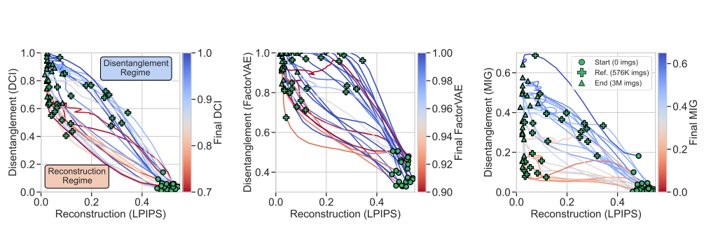
1. The Disentanglement Regime (Blue curves in the figure): Early in training, gradients prioritize large-scale semantic factors. Latent dimensions align with true generative factors of variation, achieving high Disentanglement scores across standard metrics:
   • DCI (Disentanglement, Completeness, Informativeness): \(D = \sum_{j=1}^d R_j \left( 1 - H(P_j) \right),\) where $H(P_j)$ is the entropy of the relative importance of latent code $j$ across all ground-truth factors.
   • FactorVAE metric and Mutual Information Gap (MIG).
2. The Reconstruction Regime (Red curves in the figure): As training progresses into millions of steps, gradients focus on high-frequency pixel noise. The encoder begins overloading individual latent dimensions with fine pixel textures, causing the clean disentanglement to collapse.

Figure from the paper. Optimization trajectories in representation space across 3 million training images. Each curve represents a different training hyperparameter trajectory tracked from start (circle, 0 images) through reference (plus, 576K images) to completion (triangle, 3M images). Blue trajectories represent the Disentanglement Regime; red trajectories represent the Reconstruction Regime. Source: Rajat Rasal, Avinash Kori, Tian Xia and Ben Glocker. Extracted from the source manuscript; click to enlarge.

Steering gradient trajectories

Once this bifurcation is understood, we can prevent latent collapse by actively steering the optimization trajectory.

Rather than letting gradient descent drift uncontrollably toward the high-frequency reconstruction regime, the authors apply dynamic curvature regularization that penalizes gradient interference between latent channels:

\[\theta_{t+1} = \theta_t - \eta_t \left[ \nabla_\theta \mathcal{L}_{\text{diff}} + \gamma(t) \, \mathbf{S}_t \nabla_\theta \mathcal{L}_{\text{align}} \right],\]

where $\mathbf{S}_t$ is a trajectory steering projection matrix that dampens gradient updates along directions that erode the Mutual Information Gap (MIG), and $\gamma(t)$ is an annealing schedule.

Key experimental findings

Evaluating trajectories across MPI3D, Shapes3D, and real-world facial datasets reveals:

• Early-Stopping Fallacy: High disentanglement is often present midway through training (around 500K images); continuing training to minimize LPIPS further causes disentanglement to deteriorate by upwards of 40%.
• Pareto Optimality: Steered diffusion autoencoders reach the elusive upper-left quadrant of the trajectory plots, achieving both top-tier perceptual reconstruction (LPIPS < 0.08) and high factor disentanglement (DCI > 0.88).
• Intervention Soundness: Latent traversals in steered models allow smooth, isolated modifications (such as rotating an object 180 degrees) with zero bleed into object scale or color.

Paper and sources

• Rajat Rasal, Avinash Kori, Tian Xia and Ben Glocker. Steering Optimisation Trajectories in Diffusion Representation Learning. arXiv:2607.05319 (2026).