Introduction
In any sort of brain disease, the detection of abnormality in brain image is an important task in the medical field. Brain tumors are the most common types of diseases which affect millions of peoples all over the world. The accumulation of abnormal cells leads to the formation of the tumor. The cells in the human body automatically die and get replaced with new cells, but in the case of tumors these dead cells start getting accumulated, these cells also start affecting the behavior of the normal cells in the human body. These tumors can be carcinogenic (malignant) or non-carcinogenic(benign). Tumor cells are graded based on how normal or abnormal they look, doctors will use this information to plan their treatment and surgeries, this also provides the information on the rate of growth of tumors.
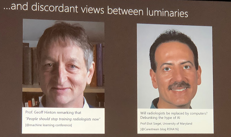
Gliomas (tumors) are rapidly progressive and neurologically devastating they affect the various functions of the brain. Common techniques used in analyzing and diagnosing these tumors if, by the mode of Magnetic resonance imaging (MRI), few other techniques include fMRI, CT, PET, ultrasound. The most widely used clinical practice is MRI based analysis. MRI is also the standard imaging modality used to delineate the brain tumor target as part of treatment planning by radiologists and surgeons. Due to the development of current technologies in the field of artificial intelligence (AI), AI can be used to a greater extent to assist doctors in treating patients. In terms of precision, the rate of analysis, repeatability and even in terms of analyzing MRI AI has achieved state-of-the-art performance which even beats doctors in some cases.
In this blog, we shall see one such robust algorithm which outperforms radiologists in terms of localizing and detecting tumors in the human brain. For the training and evaluation of this algorithm, we make use of openly available data, which was released as part of the BraTS 2018 challenge. The entire code base with trained models for segmentation can be found here Github
Data and Pre-processing
The training dataset comprises 210 high-grade glioma volumes and 75 low-grade gliomas. Each subject comprises 4 MR sequences namely FLAIR, T2, T1, T1 post-contrast. Additionally, on the training data, each subject was provided with pixel-level segmentation, Each volume of 240x240x155 dimension. A few volumes were taken along axial, few along the coronal axis, and few of them were 3D acquired sequence, So we make use of the 3D Convolutional neural network for segmentation.
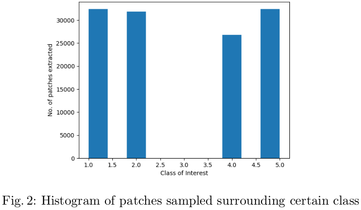
The patches of 64x64x64 were extracted. The class imbalance among the various classes in the data was circumvented by extracting a relatively more number of patches extracted from lesser frequent cases such as necrosis (class 1) were compared to edema (stratified sampling). Figure 2 illustrates the number of classes extracted around the pixel of each class.
def extract_patches(path, size = 64, stride = 6, order = 3):
    # load all volumes
    # size should be even
    seg_data   = np.uint8(nib.load(path + '_seg.nii.gz').get_data())
    flair_data = nib.load(path + '_flair.nii.gz').get_data()
    t1_data    = nib.load(path + '_t1.nii.gz').get_data()
    t1ce_data  = nib.load(path + '_t1ce.nii.gz').get_data()
    t2_data    = nib.load(path + '_t2.nii.gz').get_data()
    mask       = np.uint8(nib.load(path + 'mask.nii.gz').get_data())
    affine     = nib.load(path + '_seg.nii.gz').get_affine()
    shape      = seg_data.shape

    # normalization function...
    def normalize(img, mask):
        mean  =np.mean(img[mask !=0 ])
        std   =np.std(img[mask !=0 ])
        return (img-mean)/std

    # normalize with mask
    flair_data =normalize(flair_data, mask)
    t1_data    =normalize(t1_data, mask)
    t1ce_data  =normalize(t1ce_data, mask)
    t2_data    =normalize(t2_data, mask)

    contrasts_dict = {'flair': flair_data,
                        't1': t1_data,
                        't1ce': t1ce_data,
                        't2': t2_data}

    # normal brain tissue...
    seg_data[(mask != 0) * (seg_data <= 0)] = 5
    allowed_classes = [1, 2, 4, 5] # (5 for brain tissue, 3 is missing in data)

    # all these computations are performed for the sake of stratified sampling
    # to obtain uniform samples from all class

    arr = []
    for _class_ in allowed_classes:
        x, y, z  = np.where(seg_data == _class_)
        arr.append([len(x)])

    min_len = np.sort(np.array(arr))[::-1][-1]
    if min_len == 0:
        min_len = np.sort(np.array(arr))[::-1][-2]

    total_cntr = 0
    for _class_ in tqdm(allowed_classes):
        x_range, y_range, z_range      = np.where(seg_data == _class_)
        try:
            idx = np.random.randint(0, len(x_range),\
                                    size = min_len//stride**order)
            cntr = 0
            for (x,y,z) in zip(x_range[idx], y_range[idx], z_range[idx]):
                seg_mask = np.zeros((size, size, size))
                _mask    = np.uint8(seg_data[max(0, x-size//2 -1):min(shape[0], x+size//2 +1),
                                             max(0, y-size//2 -1):min(shape[1], y+size//2 +1),
                                             max(0, z-size//2 -1):min(shape[2], z+size//2 +1)])

                patch_info = path + 'patch_lesion_class' + str(_class_) + '_cntr' + str(cntr) + '/'

                ## SAVING REDUCED_SEG_PATCH in nii
                if _mask.shape != (size, size, size):
                    x_offset = int((size - _mask.shape[0])/2)
                    y_offset = int((size - _mask.shape[1])/2)
                    z_offset = int((size - _mask.shape[2])/2)
                    seg_mask[x_offset: x_offset + _mask.shape[0], \
                             y_offset: y_offset + _mask.shape[1], \
                             z_offset: z_offset+ _mask.shape[2]] = _mask
                else:
                    seg_mask=_mask
                save_img(path_patch + 'seg_64cube' + '.nii.gz', seg_mask, affine)

                ## SAVING REDUCED_SEQUENCE_PATCH in nii
                for contrast in contrasts_dict.keys():
                    vol_mask = np.zeros((size, size, size)) +\
                                np.min(contrasts_dict[contrast])# min background
                    vol = np.float32(contrasts_dict[contrast][max(0, x-size//2 -1):min(shape[0], x+size//2 +1),
                                                             max(0, y-size//2 -1):min(shape[1], y+size//2 +1),
                                                             max(0, z-size//2 -1):min(shape[2], z+size//2 +1)])
                    if _mask.shape != (size, size, size):
                        x_offset = int((size - vol_mask.shape[0])/2)
                        y_offset = int((size - vol_mask.shape[1])/2)
                        z_offset = int((size - vol_mask.shape[2])/2)
                        vol_mask[x_offset: x_offset + _mask.shape[0], \
                                 y_offset: y_offset + _mask.shape[1], \
                                 z_offset: z_offset+ _mask.shape[2]] = vol
                    else:
                        vol_mask=vol

                    name_scheme = contrast + '_64cube' +  '.nii.gz'
                    save_path   = os.path.join(path_patch, name_scheme)

                    if seg_mask.shape != (size, size, size) or vol_mask.shape != (size, size, size):
                        raise ValueError("alert", path, 'shape: ', seg_mask.shape)

                    save_img(save_path, vol_mask, affine)

                cntr += 1
            total_cntr += cntr
        except:
            continue
    print('patient id: ', path, 'number of patches: [', total_cntr,"]")

    pass
Segmentation Network
The segmentation network is a 3-D fully convolutional semantic segmentation network. The network accepts an input of dimension 64x64x64 and predicts the class associated to all the voxels in the input. The network comprises 57 layers. The dense connection between the various convolutional layers in the network aids in the effective reuse of the features in the network. The presence of dense connections between layers leads to requiring computational resources. This bottleneck is circumvented by keeping the number of convolutions to a small number say 4.
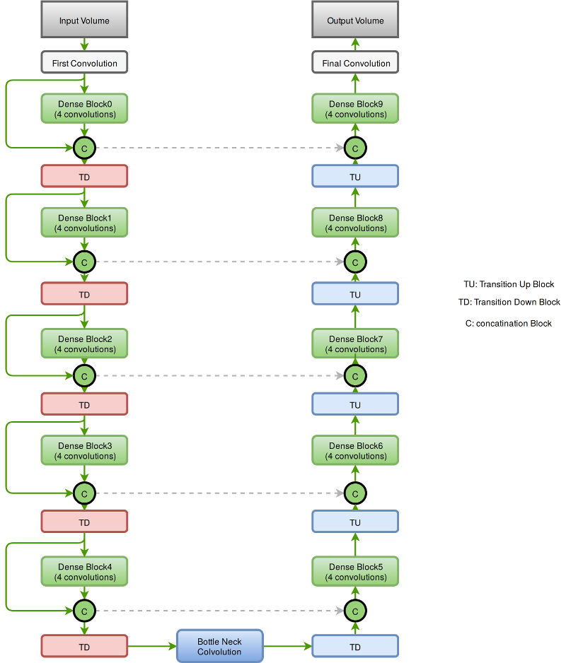
Each DenseBlock is defined by a function given below…
import torch
import torch.nn as nn

class DenseLayer(nn.Sequential):
    def __init__(self, in_channels, growth_rate):
        super().__init__()
        self.add_module('norm', nn.BatchNorm3d(in_channels))
        self.add_module('relu', nn.ReLU(True))
        self.add_module('conv', nn.Conv3d(in_channels, growth_rate, kernel_size=3,
                                          stride=1, padding=1, bias=True))
        self.add_module('drop', nn.Dropout3d(0.2))
    def forward(self, x):
        return super().forward(x)


class DenseBlock(nn.Module):
    def __init__(self, in_channels, growth_rate, n_layers, upsample=False):
        super().__init__()
        self.upsample = upsample
        self.layers = nn.ModuleList([DenseLayer(
            in_channels + i*growth_rate, growth_rate)
            for i in range(n_layers)])

    def forward(self, x):
        if self.upsample:
            new_features = []
            for layer in self.layers:
                out = layer(x)
                x = torch.cat([x, out], 1)
                new_features.append(out)
            return torch.cat(new_features,1)
        else:
            for layer in self.layers:
                out = layer(x)
                x = torch.cat([x, out], 1)
            return x
Training & Testing
The network was trained by minimizing weighted cross-entropy, (The weight associated to each class was equivalent to the ratio of the median of the class frequency to the frequency of the class of interest) and the learning rate was initialized to 0.0001 and decayed by a factor of 10 % every-time the validation loss plateaued.
#-------------------- SETTINGS: OPTIMIZER & SCHEDULER
optimizer = optim.Adam (model.parameters(), lr=learningRate, betas=(0.9, 0.999), eps=1e-05, weight_decay=1e-5)
scheduler = ReduceLROnPlateau(optimizer, factor = 0.1, patience = 5, mode = 'min')

#-------------------- SETTINGS: LOSS
weights = torch.FloatTensor([9.60027345, 0.93845396, 1.02439363, 1.00,    0.65776251]).to(device)
CE_loss = torch.nn.CrossEntropyLoss(weight = weights)

loss = CE_loss + dice_loss
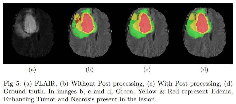
During inference, patches of the dimension of 64x64x64 were extracted from the volume and fed to the network. CNN’s being a deterministic technique is bound to generate predict the presence of a lesion in a physiological impossible place. The false positives generated by the network were reduced by performing conditional random fields (CRF), these false positives were further reduced by performing the 3-D connected component analysis.
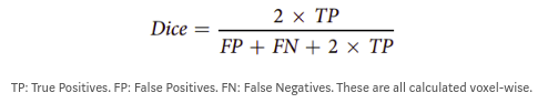
The Dice Score
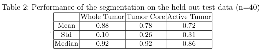
Due to the huge class imbalance, a regular accuracy score does not say a lot. Thus, for each category, the common F1 score is used (in the literature known as the Dice score). It measures the overlap between manual segmentation (the combination of expert raters’ opinion: the fused score) and the machine learning segmentation.
Dice loss = 1.0 - DiceScore
def dice_loss(input,target):

    target = to_one_hot(target, n_dims=nclasses).to(device)

    assert input.size() == target.size(), "Input sizes must be equal."
    assert input.dim() == 5, "Input must be a 5D Tensor."

    probs = F.softmax(input)

    num   = (probs*target).sum() + 1e-3
    den   = probs.sum() + target.sum() + 1e-3
    dice  = 2.*(num/den)
    return 1. - dice
Conclusion
Artificial intelligence has a lot of potential in the healthcare industry. These deep learning models being deterministic in nature once trained will always provide the same results for a given input, which isn’t the case with radiologists (reduce intra-class variability). Based on the above results, semantic segmentation through deep learning clearly has a huge advantage in neurology, neurosurgery and many other health problems. It will enable us to diagnose various brain diseases and track their progression which is essential for effective treatment. AI-assisted health care is of huge interest and is a lot smarter and efficient.
Feel free to add comments and also share your thoughts…
Leave a Comment