
Optimization, one of the most interesting topics in the field of General Artificial Intelligence. Most of the problems we encounter in our daily life are solved by numerical optimization methods. Here in this blog, let us look back on some basic numerical optimization algorithms extensively in finding local optima of any given function (one which works best with convex functions). Let’s start with simple convex functions, where local and global minima are one and the same, and move towards highly non-linear functions with multiple local and global minima’s. Entire optimization revolves around basic concepts of linear algebra and differential calculus. Recent updates in deep learning have created huge interest in the field of numerical and stochastic optimization algorithms, to provide theoretical backing for amazing qualitative results shown by deep learning algorithms. In these kinds of learning algorithms, there isn’t any explicitly known function for optimization, but we only have access to the 0th and 1st order oracles. Oracles are the black boxes which return function value, gradient or Hessian of the function at any given point. 0th order oracle returns function value, while 1st order oracle returns the gradient value of a function. This blog provides the basic theoretical and numerical understanding of unconstrained optimization functions and also includes a python implementation of them.
Necessary and sufficient conditions for a point to be a local minima:
For any point to be minima it should satisfy the following conditions: \(f(x^*) \leq f(x) \quad \quad \forall x \in R^d\)
Let f(.) be a continuous and twice differentiable function
First order nescessary condition
\[\nabla f(x^*) = 0\]Second order nescessary condition
\[\nabla f(x^*) = 0\] \[\nabla ^2 f(x^*) \succcurlyeq 0\]Second order sufficiency condition
\[\nabla f(x^*) = 0\] \[\nabla ^2 f(x^*) \succ 0\]Gradient Descent;
Gradient descent is the backbone for all the advancements in the field of learning algorithms (machine learning, deep learning or deep reinforcement learning). In this blog, we shall see the various modifications on gradient descent for faster and better convergence. Let us consider the case of linear regression where we estimate the coefficients of the equation: \(y = \theta_0 + \theta_1 x_1 + ... + \theta_n x_n\). Assuming the function to be the linear combination of all features. The optimal set of coefficients is determined by minimizing \(||y - \theta^T X||^2\) loss function, which turns out to be the maximum likelihood estimate for the task of linear regression. Minimizing OLS (Ordinary least Square) involves finding the inverse of feature matrix \(\theta^* = [XX^T]^{-1}XY\)
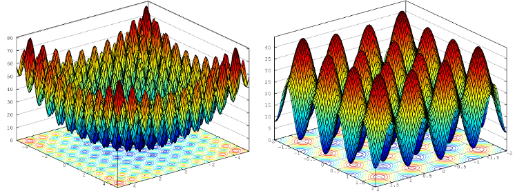
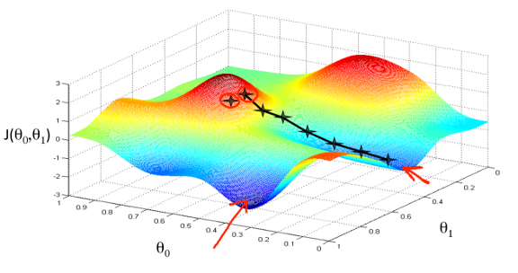
For a practical problem, the dimensionality of the data is huge which would easily blow up the computational power. For example, let us consider the problem of image feature analysis: generally images are of size 1024x1024 which means the number of features is of the order \(10^6\). Due to a large number of features, such optimization problems are solved in an iterative way, and this leads us to the very popularly known algorithm called gradient descent and Newton-raphson method.
Gradient Descent Algorithm:
\[X \leftarrow X - \eta \nabla f(X)\] \[X_{t+1} = X_{t} - \eta \nabla f(X_t)\]Gradient descent algorithm updates an iterate in the direction of the negative gradient (hence, the steepest descent direction) with a previously specified learning rate \(\eta\). The learning rate is used to prevent the overshoot of the local minima at any given iteration.
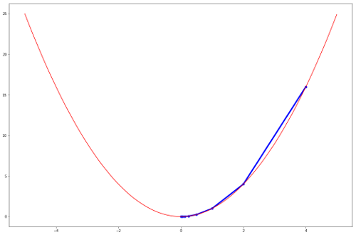
Below figure shows convergence of gradient descent algorith for function \(f(x) = x^2\) with \(\eta = 0.25\)
Finding out an optimal \(\eta\) is the task at hand, which requires the prior knowledge of functions under study and the domain of operation.
# python implementation of vanilla gradient descent update rule
def gradient_descent_update(x, eta):
    """
        get_gradient is 1st order oracle
    """
    return x - eta*get_gradient(x)
Gradient Descent with Armijo Goldstein condition:
To reduce the work of setting \(\eta\) manually, Armijo Goldstein (AG) conditions are applied to find \(\eta\) for the next iteration. Formal derivation of AG condition requires the knowledge of linear approximation, Lipchitz conditions, and basic calculus, which are beyond the context of this explanation.
\[X_{t+1} = X_{t} - \eta \nabla f(X_t)\]Let’s define two functions \(f_1(x)\) and \(f_2(x)\) as linear approximation of \(f(x)\) with two different coefficients \(\alpha \& \beta\)
\[f_1(X_{t+1}) = f(X_t) - \eta \alpha |\nabla f(X_t)|^2\] \[f_2(X_{t+1}) = f(X_t) - \eta \beta |\nabla f(X_t)|^2\]In each iteration of the AG condition, a specific \(\eta\) which satisfies relation \(f_1(X_{t+1}) \leq f(X_{t+1}) \leq f_2(X_{t+2})\) is found and the curent iterate is updated accordingly. Below figure shows the range of next iterate, for the convergence of function \(f(x) = x^2\) with \(\alpha = 0.25\) and \(\beta = 0.5\) :
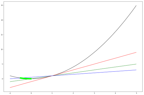 Red, Blue and Green line in the above figure corresponds to \(f(x), \quad f_1(x) \quad \& \quad f_2(x)\), The band of lightgreen show’s the range of next possible iterate.
# python implementation of vanilla gradient descent with AG condition update rule
def gradient_descent_update_AG(x, alpha=0.5, beta=0.25):
    eta=0.5
    max_eta=np.inf
    min_eta=0.
    value = get_value(x)
    grad  = get_gradient(x)
    while True:
        x_cand = x - (eta)*grad
        f  = get_value(x_cand)
        f1 = value - eta*alpha*np.sum(np.abs(grad)**2)
        f2 = value - eta*beta *np.sum(np.abs(grad)**2)
        if f<=f2 and f>=f1:
            return x_cand
        if f>f2:
            max_eta = eta
            eta = (eta+min_eta)/2.0
        if f<f1:
            min_eta = eta
            eta = np.min(2.*eta, (eta+max_eta)/2.)
Gradient Descent with Full Relaxation condition:
In the case of Full relaxation condition, new a function \(g(\eta)\) is minimized to obtain \(\eta\) which is subsequently used to find next iterate.
\[g(\eta) = f(X - \eta \nabla f(X))\] \[\eta* = argmin (g(\eta))\]This method involves solving the optimization problem for finding every next iterate, which is done as:
\[g'(\eta) \rightarrow 0\] \[\nabla f(X - \eta \nabla f(X))*\nabla f(X) \rightarrow 0\]The python implementation for the above is shown below:
def gradient_descent_update_FR(x):
    eta     = 0.5
    thresh  = 1e-6
    max_eta = np.inf
    min_eta = 0.

    while True:
        x_cand = x - eta*get_gradient(x)
        g_diff = -1.*get_gradient(x)*get_gradient(x_cand)

        if np.sum(np.abs(g_diff)) < thresh and eta > 0:
            return x_cand

        if  eta < eta_min:
            min_eta = eta
            eta = min(2.*eta, (eta+max_eta)/2.)
        else:
            max_eta = eta
            eta = (eta+min_eta)/2.
Stochastic Gradient Descent
As we know, in a real setup the dimension of the data will be quite huge which makes further gradient computation for all the features expensive. In such cases, a random batch of points (features) are selected and the expected gradient is computed. This whole setup convergence only in an expectational sense.
Mathematically it would mean:
Randomly select a point (p) for estimating gradients.
\[X_{t+1} = X_{t} - \eta (\frac{1}{m} \Sigma_i^m \nabla f_i(X_t) + {\nabla f_p(X_t) - \frac{1}{m} \Sigma_i^m \nabla f_i(X_t)}\]Let, \(w_t = \nabla f_p(X_t) - \frac{1}{m} \Sigma_i^m \nabla f_i(X_t)\)
\[X_{t+1} = X_{t} - \eta (\frac{1}{m} \Sigma_i^m \nabla f_i(X_t) + w_t\]In the above iterate \(w_t\) can be treated as noise. This iterate leads towards local optima only when \(E(w_t) \rightarrow 0\)
Let the probability of selecting the random feature point \((f_p)\) be \(\frac{1}{m}\)
\[E(w_t) = E( \nabla f_p(X_t) - \frac{1}{m} \Sigma_i^m \nabla f_i(X_t))\] \[\Rightarrow E( \nabla f_p(X_t)) - E(\frac{1}{m} \Sigma_i^m \nabla f_i(X_t))\] \[\Rightarrow E(\nabla f_p(X_t)) - \frac{1}{m} \Sigma_i^m \nabla f_i(X_t)\] \[\Rightarrow 0\]Similarly, it can be shown that a variance of \(w_t\) is also finite. By the above proof, the convergence of SGD is guaranteed.
Python implementation of SGD is given below
def SGD(self, X, Y, batch_size, thresh=1):
        loss = 100
        step = 0
        if self.plot: losses = []

        while loss >= thresh:
            # mini_batch formation
            index = np.random.randint(0, len(X), size = batch_size)
            trainX, trainY = np.array(X)[index], np.array(Y)[index]

            self.forward(trainX)
            loss = self.loss(trainY)
            self.gradients(trainY)

            # update
            self.w0 -= np.squeeze(self.alpha*self.grad_w0)
            self.weights -= np.squeeze(self.alpha*self.grad_w)

            losses.append(loss)
            if step % 1000 == 999: print "Batch number: {}".format(step)+" current loss: {}".format(loss)
            step += 1
        if self.plot : self.visualization(X, Y, losses)
        pass
AdaGrad
Adagrad is an optimizer that helps in the automatic adaptation of the learning rate for each and every feature involved in the optimization problem. This is achieved by keeping the track of the history of all the gradients. This method also converges only in the expectation sense.
the python implementation is shown below :
def AdaGrad(self, X, Y, batch_size, thresh = 0.5, epsilon = 1e-6):
        loss = 100
        step = 0
        if self.plot: losses = []
        G = np.zeros((X.shape[1], X.shape[1]))
        G0 = 0
        while loss >= thresh:
            # mini_batch formation
            index = np.random.randint(0, len(X), size = batch_size)
            trainX, trainY = np.array(X)[index], np.array(Y)[index]

            self.forward(trainX)
            loss = self.loss(trainY)
            self.gradients(trainY)

            G += self.grad_w.T*self.grad_w
            G0 += self.grad_w0**2
            den = np.sqrt(np.diag(G)+epsilon)

            delta_w = self.alpha*self.grad_w / den
            delta_w0 = self.alpha*self.grad_w0 / np.sqrt(G0 + epsilon)

            # update parameters
            self.w0 -= np.squeeze(delta_w0)
            self.weights -= np.squeeze(delta_w)

            losses.append(loss)
            if step % 500 == 0: print "Batch number: {}".format(step)+" current loss: {}".format(loss)
            step += 1
        if self.plot : self.visualization(X, Y, losses)
        pass
Let us move towards Hessian based methods, Newton and quasi-Newton method:
Update rule for Newton’s method is defined as:
\[X \leftarrow X - [\nabla^2 f(X)]^{-1} \nabla f(X)\]The convergence of this algorithm is much faster than gradient-based methods. Mathematically, convergence rate of gradient descent is proportional to \(O(\frac{1}{t})\), while for Newton’s method it is proportional to \(O(\frac{1}{t^2})\). But in case of higher-dimensional data, estimating 2nd order oracle for each iterate is computationally expensive, leading to the 2nd order oracle being simulated using the 1st order oracle. This gives us the quasi-Newton class of algorithms. The most frequently used algorithm in this class of quasi-Newton method is the BFGS and LMFGS algorithm. In this blog, we only discuss the BFGS algorithm which involves rank one matrix update of the Hessian of the function. The overall idea of the method is to randomly initialize the Hessian and keep updating the Hessian with each iteration using a rank-one update rule.
Mathematically this is shown as:
Let : \(s_t = X_{t+1} - X_t\), \(y_k = \nabla f(X_{t+1} - \nabla f(X_t)\) and \(H_t\) be Hessian inverse estimate of the function for \(t^th\) iteration.
Let \(\rho_t = \frac{1}{s_t^Ty_t}\) be the normalizing term
\[X_{t+1} = X_t - H_t \nabla f(X_t)\] \[H_{t+1} = (I - \rho_t s_t y_t^T)H_t(I - \rho_t y_t s_t^T) + \rho_t s_t s_t^T\]This rule can be derived using Lipchitz conditions of smoothness and continuity and \(H_t \in S_{++}\) at every iteration.
Python implementation for BFGS is given below:
def BFGS_update(H, s, y):
    smooth = 1e-3
    s   = np.expand_dims(s, axis= -1)
    y   = np.expand_dims(y, axis= -1)
    rho = 1./(s.T.dot(y) + smooth)
    p   = (np.eye(H.shape[0]) - rho*s.dot(y.T))
    return p.dot(H.dot(p.T)) + rho*s.dot(s.T)

def quasi_Newton(x0, H0, num_iter=100, eta=1):
    xo, H = x0, H0
    for _ in range(num_iter):
        xn = xo - eta*H.dot(get_gradient(xo))
        y = get_gradient(xn) - get_gradient(xo)
        s = xn - xo
        H = BFGS_update(H, s, y)
        xo = xn
    return xo
For more deeper understanding refer to:
- Numerical Optimization (by Jorge Nocedal and Stephen J. Wright)
- Nonlinear Programming by Yu Nestrov
The entire code used in this post can be found here
Leave a Comment