
In my previous blog, I had discussed unconstrained optimization problems and methods involved to solve them. In this blog, we shall discuss a few key concepts revolving around constrained optimization (which includes problem formulation and solving strategies). This blog also discusses the theory and Python implementation of an algorithm known as SVM (Support Vector Machine).
When we come across real-life problems, coming up with an ideal optimization function is quite hard and sometimes not feasible, so we relax on optimization function by imposing additional constraints on the problem, and optimizing this constrained setup would provide an approximation which we would be as close a possible to the actual solution of the problem, but would also be feasible. To solve constrained optimization problems methods like Lagrangian formulation, penalty methods, projected gradient descent, interior points, and many other methods are used. In this blog post, we’ll go through Lagrangian formulation and projected gradient descent. This blog post also covers the details about open-source toolbox used for optimization CVXOPT, and also covers SVM implementation using this toolbox.
General form of constrained optimization problems:
\[min_x f(x)\] \[s.t \quad g(x) \leq 0\] \[h(x) = 0\]where \(f(x)\) is the objective function, and \(g(x)\) and \(h(x)\) are inequality and equality constraints respectively. If \(f(x)\) is convex and the constraints form a convex set, (i.e g(x) is convex and h(x) is affine), the optimization is guaranteed to converge at a global minima. For any other set of problems, it converges to local minima.
Projected gradient descent
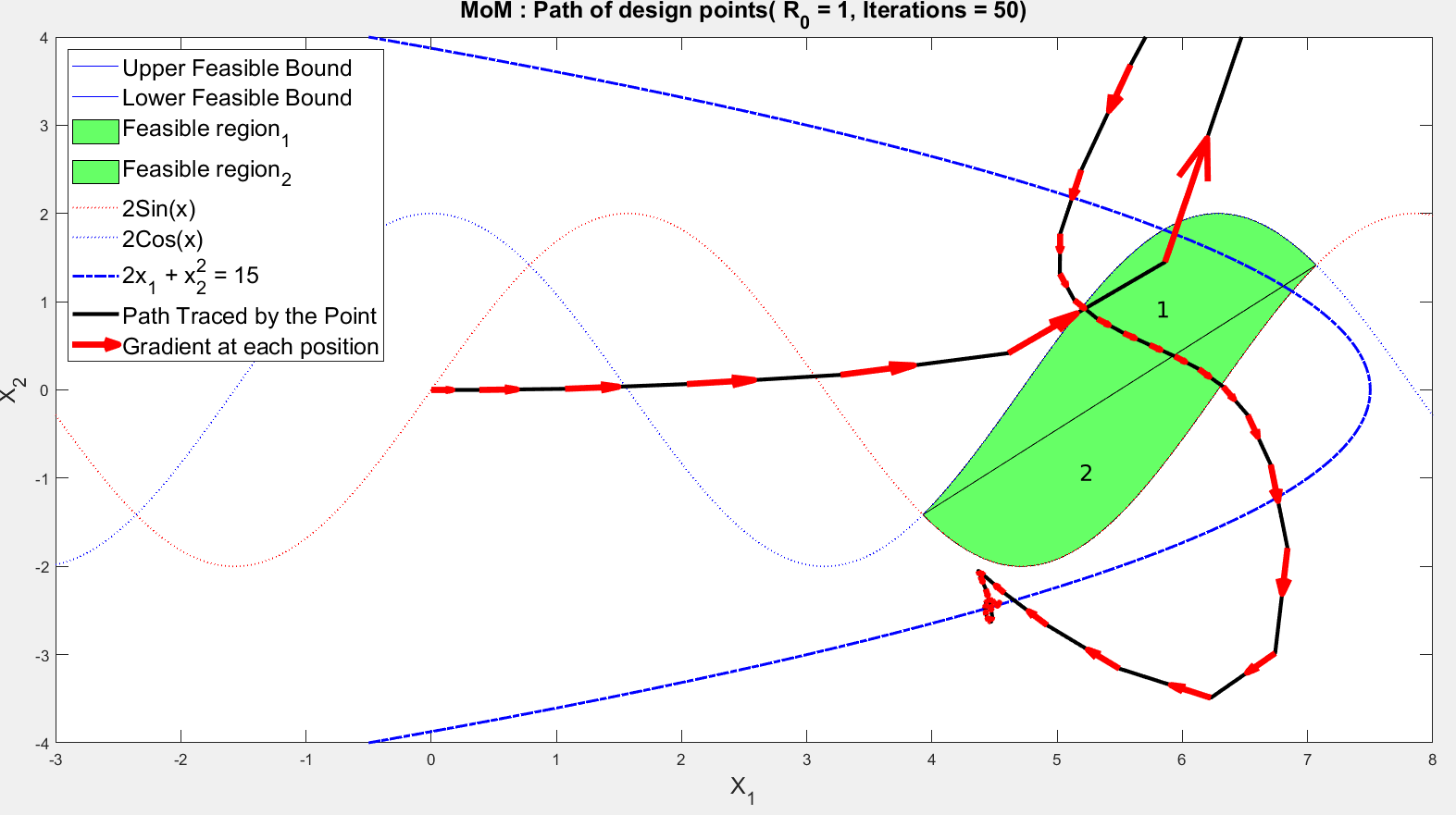
The preliminary(and most obvious) step while solving constrained optimization setup is to take the projection of an iterate over a constrained set. This turns out to be the most powerful algorithm in solving the constrained optimization problem. This involves two steps (1) to find the next possible iterate in minimization (descent) direction, (2) Finding projection of the iterate on constrained set.
-
step1: \(\hat x_{t+1} \leftarrow x_t + \eta P_t\) where \(P_t\) is descent direction
-
step2: \(x_{t+1} \leftarrow \Pi_A(\hat x_{t+1})\) where \(\Pi\) is projection oracle and set A is constraints set in general \(\Pi_A (x_0) = argmin_{x \in A} \|\| x - x_0\|\|^2\)
Python implementation of projected gradient descent on l1 and l2 norm constrained the set
def projection_oracle_l2(w, l2_norm):
    return (l2_norm/np.linalg.norm(w))*w

def projection_oracle_l1(w, l1_norm):
    # first remeber signs and store them. Modify w
    signs = np.sign(w)
    w = w*signs
    # project this modified w onto the simplex in first orthant.
    d=len(w)
    if np.sum(w)<=l1_norm:
        return w*signs

    for i in range(d):
        w_next = w+0
        w_next[w>1e-7] = w[w>1e-7] - np.min(w[w>1e-7])
        if np.sum(w_next)<=l1_norm:
            w = ((l1_norm - np.sum(w_next))*w + (np.sum(w) - l1_norm)*w_next)/(np.sum(w)-np.sum(w_next))
            return w*signs
        else:
            w=w_next
def main():
    eta=1/smoothness_coeff
    for l1_norm in np.arange(0,10,0.5):
        w=np.random.randn(data_dim)
        for i in range(1000):
            w = w - eta*get_gradient(w)
            w = projection_oracle_l1(w, l1_norm)
    pass
Understanding Lagrangian formulation
In most of the optimization problems, finding the projection of an iterate over a constrained set is a difficult problem (especially in the case of a complex constrained set). It is similar to solving an optimization problem at each iterate, which would be non-convex in most of the cases. In reality, people try to get rid of the constraints by solving the dual problem rather than the primal problem.
Before diving into Lagrangian dual and primal formulation let’s understand KKT conditions and it’s significance
-
For any point to be local\global minima with equality constraints: \(\nabla f(x) = \mu \nabla h(x), \mu \in R\)
-
Similarly in case of inequality constraints: \(\nabla f(x) = -\lambda \nabla g(x), \lambda \in R_+\)
These two conditions can be easily observed by considering a unit circle as a constrained set. In the first part, let us consider only a boundary where the sign of \(\mu\) doesn’t matter, this is the result of equality constraints. In the second case, consider an interior set of a unit circle where -ve sign for \(\lambda\) signifies the feasible solution region.
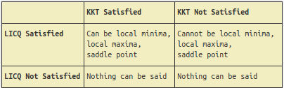
KKT (Karush–Kuhn–Tucker) conditions are considered as first-order necessary conditions, which a point should satisfy to be considered as a stationary point (local minima, local maxima, saddle point. For \(x^*\) to be local minima:
-
\(g_i(x^*) \leq 0\) and \(h_i(x^*) = 0\)
-
\(\nabla f(x^*) = \Sigma \mu_i \nabla h_i(x^*) - \Sigma \lambda_j \nabla g_j(x^*)\) for all \(\mu_i \in R\) and \(\lambda_i \in R_+\)
-
\(\lambda_i g_i(x^*) = 0\) Active constraints conditions
LICQ condition: all active constraints \((h_j(x^*) = 0, g_i(x^*) = 0)\) should be linearly independent of each another
Lagrangian of a function
For any function \(f(x)\) with inequality constraints \(g_i(x) \leq 0\) and equality constraints \(h_i(x) = 0\) , Lagrangian \(L(x, \lambda, \mu)\) for all \(\mu_i \in R\) and \(\lambda_i \in R_+\) is defined as:
\[L(x, \lambda, \mu) = f(x) + \lambda_i g_i(x) + \mu h_i(x)\] \[min_x f(x)\] \[s.t \quad g(x) \leq 0\] \[h(x) = 0\]above optimization is equivalent to :
\[min_x max_{\lambda \in R+, \mu \in R} L(x, \lambda, \mu)\]Above formulation is known as the primal problem \(p^*\) by the claim of game theory (i.e second player will always have a better chance for optimization) it can be easily seen that:
\[max_{\lambda \in R+, \mu \in R} min_x L(x, \lambda, \mu) \leq min_x max_{\lambda \in R+, \mu \in R} L(x, \lambda, \mu)\]\(max_{\lambda \in R+, \mu \in R} min_x L(x, \lambda, \mu)\), This formulation is known as the dual problem \((d^*)\).
Both primal and dual formulations lead to the same optimal value if and only if the objective function \(f(x)\) is convex and the constrained set is also convex. Proof of this claim is justified below:\
let the function be convex which implies \(L(x^*, \lambda, \mu) \leq L(x, \lambda, \mu)\)
\[max_{\lambda \leq 0, \mu} min_x L(x, \lambda, \mu) \geq min_x L(x, \lambda^*, \mu^*) = L(x^*, \lambda^*, \mu^*)\] \[min_x max_{\lambda \leq 0, \mu} L(x, \lambda, \mu) \leq max_{\lambda \leq 0, \mu} L(x^*, \lambda, \mu) = L(x^*, \lambda^*, \mu^*)\]based on the above two equations:
\[max_{\lambda \leq 0, \mu} min_x L(x, \lambda, \mu) = min_x max_{\lambda \leq 0, \mu} L(x, \lambda, \mu)\]SVM (Support Vector Machines)
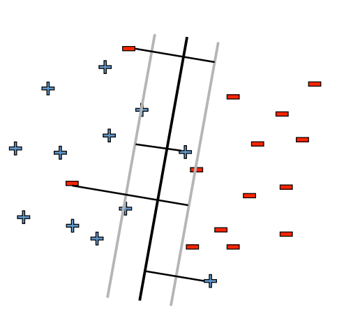
SVM’s belong to a supervised learning class of algorithms used in classification and regression problems. SVM’s are easily scalable and can solve linear and non-linear problems (by making use of kernel-based trick). In most of the problems, we can’t draw a single line differentiating two different class of data, due to which we need to provide a slight margin in the construction of decision boundaries, which is easily formulated using SVM. The idea of SVM is to create the separating hyperplane between two different sets of data points. Once the separating hyperplane is obtained, it becomes relatively easier to classify data points (test case) in one of the classes. SVM works well even for higher-dimensional data. The advantages of SVM’s are that they are memory efficient, accurate and fast as compared with other ML models. Let’s look at the mathematics of SVM …
SVM with Primal Objective
\[min_{w \in R^d, \xi \in R^n} \frac{1}{2}||w||^2 + c\Sigma_{i=1}^n \xi_i\] \[s.t \quad (w.x_j+b)y_j \geq 1-\xi_j \forall j\] \[\xi_j \geq 0 \forall j\]As SVM objective is convex in nature primal and dual results in same optimal solution.
SVM Dual Objective
\[max_\lambda -\frac{\lambda^T YKY \lambda}{2} + I^T \lambda\] \[s.t\quad 0\leq \lambda_i \leq c\] \[\Sigma \lambda_i y_i = 0\]Derivation of SVM Dual
\[p^* = min_{w\in R^d} max_{\lambda, \mu} L(w, \lambda, \mu)\] \[\Rightarrow min_{w\in R^d} max_{\lambda \in R_+, \mu \in R} \frac{1}{2}||w||^2 + c\Sigma_{i=1}^n \xi_i + \lambda_1 (1-\xi -(w.x_j+b)y_j) - \lambda_2 \xi_j\]Lagrangian formulation …
\[d^* = max_{\lambda, \mu} min_{w\in R^d} L(x, \lambda, \mu)\] \[\Rightarrow max_{\lambda \in R_+, \mu \in R} min_{w\in R^d} \frac{1}{2}||w||^2 + c\Sigma_{i=1}^n \xi_i + \lambda_1 (1-\xi -(w.x_j+b)y_j) - \lambda_2 \xi_j\] \[\phi(\lambda) = L(w^*, \lambda)\]where \(w^*\) is such that:
\[\nabla_w^* (\frac{1}{2}||w||^2 + c\Sigma_{i=1}^n \xi_i + \lambda_1 (1-\xi -(w.x_j+b)y_j) - \lambda_2 \xi_j) = 0 \quad for \quad minima\]\(\phi(\lambda) = -\inf\) if \(\Sigma \lambda_i y_i \neq 0\) or\(\lambda_i \leq c\)
\[\phi(\lambda) \frac{-1}{2}(\Sigma \lambda_i x_i y_i)^T(\Sigma \lambda_i x_i y_i) + \Sigma \lambda_i\] \[\Rightarrow \frac{-1}{2}(\lambda y)^T K (\lambda y) + \Sigma \lambda\]where \(K \in R^{n \times n}\) such that \(K_{ij} = x_i ^T x_j\) and \(Y \in R^{n \times n}$ and $Y = diag(y)\)
\[\Rightarrow \frac{-1}{2}\lambda^T Y K Y\lambda + \Sigma \lambda\]This leads to the dual problem as:
\[max_\lambda -\frac{\lambda^T YKY \lambda}{2} + I^T \lambda\] \[s.t\quad 0\leq \lambda_i \leq c\] \[\Sigma \lambda_i y_i = 0\]CVXOPT
In the section, we’ll discuss the implementation of the above SVM dual algorithm in python using the CVXOPT library. You can find more about library here
General CVXOPT format for such problems
\[min_x \frac{1}{2}x^T P x + q^T x\] \[s.t \quad Gx + s = h\] \[Ax = b\]import numpy as np
from cvxopt import matrix, solvers
def solve_SVM_dual_CVXOPT(x_train, y_train, x_test):
"""
Solves the SVM training optimization problem (the dual) using cvxopt.
Arguments:
x_train: A numpy array with shape (n,d), denoting n training samples in \R^d.
y_train: numpy array with shape (n,) Each element takes +1 or -1
x_train: A numpy array with shape (m,d), denoting m test samples in \R^d.
Limits:
n<200, d<100, m<1000
Returns:
y_pred_test: A numpy array with shape (m,). This is the result of running the learned model on the test instances x_test. Each element is +1 or -1.
"""
n, d = x_train.shape
c = 10 # let max \lambda value be 10
y_train = np.expand_dims(y_train, axis=1)*1.
P = (y_train * x_train).dot((y_train * x_train).T)
q = -1.*np.ones((n, 1))
G = np.vstack((np.eye(n)*-1,np.eye(n)))
h = np.hstack((np.zeros(n), np.ones(n) * c))
A = y_train.reshape(1, -1)
b = np.array([0.0])
P = matrix(P); q = matrix(q)
G = matrix(G); h = matrix(h)
A = matrix(A); b = matrix(b)
sol = solvers.qp(P, q, G, h, A, b)
lambdas = np.array(sol['x'])
w = ((y_train * lambdas).T.dot(x_train)).reshape(-1,1)
b = y_train - np.dot(x_train, w)
prediction = lambda x, w, b: np.sign(np.sum(w.T.dot(x) + b))
y_test = np.array([prediction(x_, w, b) for x_ in x_test])
return y_test
if __name__ == "__main__":
# Example format of input to the functions
n=100
m=100
d=10
x_train = np.random.randn(n,d)
x_test = np.random.randn(m,d)
w = np.random.randn(d)
y_train = np.sign(np.dot(x_train, w))
y_test = np.sign(np.dot(x_test, w))
y_pred_test = solve_SVM_dual_CVXOPT(x_train, y_train, x_test)
check1 = np.sum(y_pred_test == y_test)
print ("Score: {}/{}".format(check1, len(y_Test)))
For more deeper understanding refer to:
- Numerical Optimization (by Jorge Nocedal and Stephen J. Wright)
- Nonlinear Programming by Yu Nestrov
The entire code used in this post can be found here
Leave a Comment