
Maritime Motion Foundation Models: AIS, Latent Dynamics, and Compositional Coverage
In brief
- Observation: AIS records are partial observations of underlying vessel states and reporting processes; physical drivers and measurement errors are not fully observed.
- Coverage: Pretraining needs more than diverse AIS messages. Marginal, compositional, and dynamical coverage address different gaps; synthetic scenarios can deliberately expand feasible combinations.
- Foundation: Broad pretraining and adaptability are central to the foundation-model claim. Reuse across tasks, regions, vessels, and observation regimes must be demonstrated.
A vessel approaches a channel junction. Its recent AIS reports are known, but immediate navigational intent, currents, propulsion settings, and reporting errors may not be. Two different future routes can fit the same history. A predictor that averages those routes may produce a path that follows neither navigable branch. The task is therefore to represent possible futures and their uncertainty, not merely a single best continuation.
This example raises a broader question: what should an AIS based maritime motion foundation model learn? Foundation models are broadly pretrained and adaptable to multiple downstream tasks (Bommasani et al., 2021). For maritime motion, the argument is that a reusable base should capture regularities across physical motion, observation regimes, and feasible combinations of operating conditions. Broad pretraining and adaptability across tasks are central to the foundation-model concept. For maritime motion, this claim needs evidence that the learned base transfers across meaningful tasks and operating regimes.
The probabilistic formulation below is a proposed modelling perspective, not a claim that AIS reveals every physical driver or that an existing simulator has exhaustive coverage.
1. AIS Is an Observation, Not the Vessel State
Distinguish the underlying physical state \(S_t\) from a reported AIS position \(X_t^{\mathrm{obs}}\). The physical state may include true position, velocity, heading, and other motion variables; it is not directly observed in full in an AIS-only archive. An AIS position can be an accurate proxy for true position, but the received report is still a measurement, not a complete physical description.
AIS may report position, speed over ground, course, heading, identity, and other metadata, depending on equipment and data availability (US Coast Guard). Speed over ground is not a direct measurement of propulsion effort or current velocity. Currents, wind, response parameters, control actions, and navigational intent should not be treated as measured inputs when only AIS is available.
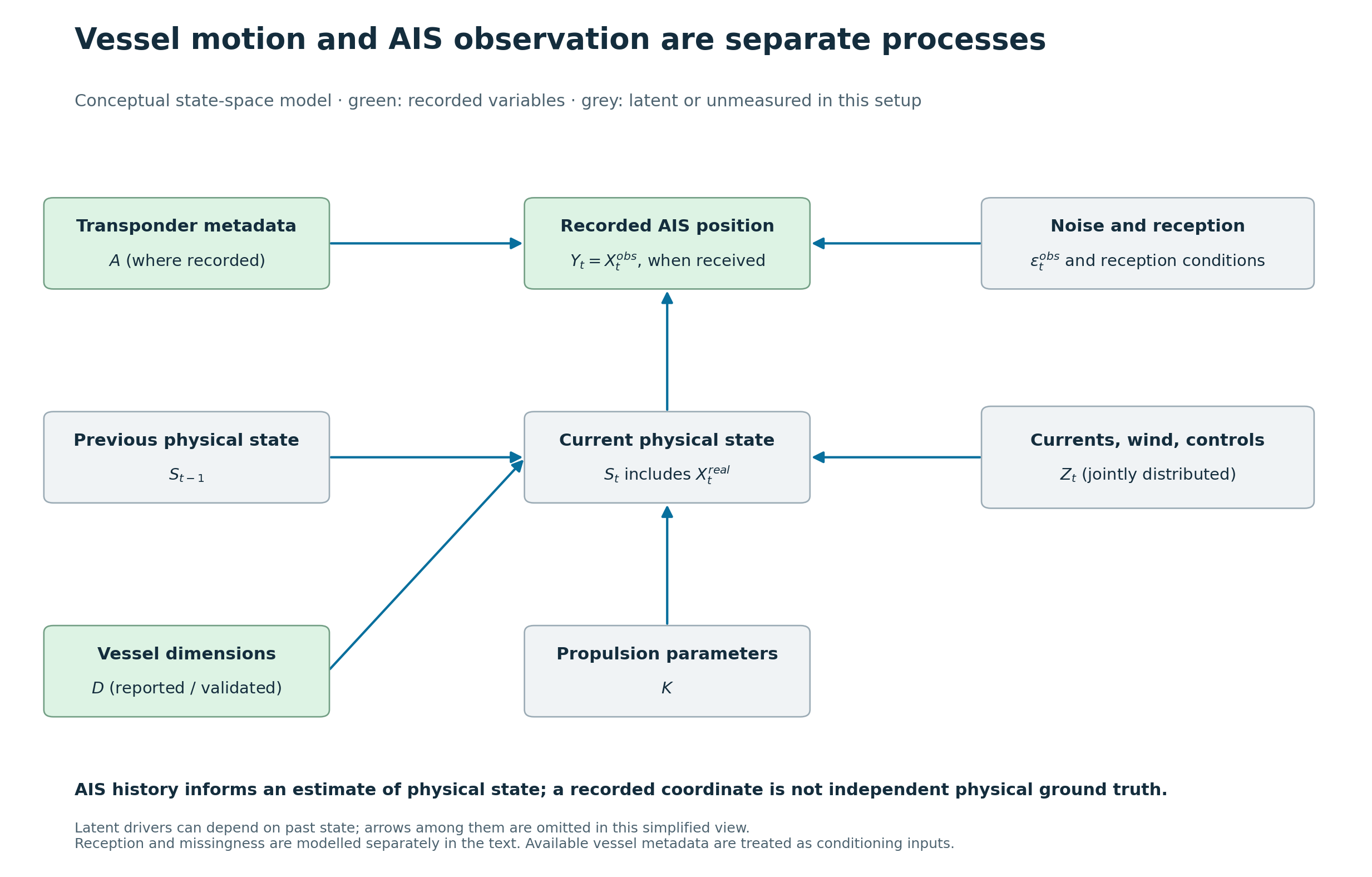
Let \(D\) denote vessel dimensions, \(A\) observed transponder metadata, \(K\) latent vessel response or propulsion parameters, and \(Z_t\) time-varying latent drivers such as environmental forcing and control decisions. A conceptual state-space formulation is:
\[\begin{aligned} S_t &= F(S_{t-1}, Z_t, D, K, \Delta t;\epsilon_t^{\mathrm{dyn}}),\\ X_t^{\mathrm{obs}} &= G(S_t, A, Z_t;\epsilon_t^{\mathrm{obs}}), \quad \text{when a usable report is received}. \end{aligned}\]The transition \(F\) models motion; \(G\) models observation. Their noise terms differ, and \(\Delta t\) matters because AIS observations are irregularly spaced. Nominal AIS transmission intervals depend on equipment class, speed, and course changes (US Coast Guard; IALA). Reception gaps introduce another source of irregularity. Conceptually distinguish a transmission indicator \(R_t^{\mathrm{tx}}\) from a reception or dataset-availability indicator \(R_t^{\mathrm{rx}}\). In a received AIS archive, only the latter is directly reflected in the available records; absent reports do not establish whether the vessel transmitted. Below, \(R_t\) denotes dataset availability on a specified analysis grid, not observed transmission.
A learned AIS model fits a distribution over available observations after latent variables have been marginalised. Good observational likelihood does not identify wind, engine response, current, or intent uniquely. External measurements, structural assumptions, constraints, or interventions are needed to distinguish competing mechanisms. Where radar or reference-grade positioning is available, it provides another observation with its own error model.
2. Maritime Futures Are Distributions
Let \(H_t\) include received AIS history, elapsed time intervals, available metadata, and report masks up to \(t\). A probabilistic forecasting model can target both future reports and their availability:
\[q_\theta(Y_{t+1:t+H},R_{t+1:t+H}\mid H_t).\]Alternatively, a model may forecast physical or interpolated positions at selected times, but that requires a clearly stated prediction target and observation-time convention.
At a junction, two branches may both be plausible. A conditional mean of those trajectories may pass between the branches, matching neither feasible route. A useful forecast must therefore preserve distinct route modes as well as uncertainty within each mode. TrAISformer is one published example of AIS trajectory prediction using a discretised representation and cross-entropy training to address heterogeneous trajectory outcomes (Nguyen and Fablet, 2024).
Several sources of uncertainty should remain conceptually separate: ambiguous future decisions, unobserved forcing, sensor or reporting error, and sparse coverage of a regime in training. A point forecast or uncalibrated probability distribution can conceal these differences.
3. Historical AIS Does Not Guarantee Coverage
Historical archives repeatedly sample the fleets, seasons, routes, operational practices, and receiving infrastructures that happened to be observed. Increasing the number of messages in common regimes does not necessarily teach a model what happens under rare but feasible combinations.
We propose three complementary dimensions of coverage for maritime motion pretraining:
| Coverage type | What it captures | Example failure when missing |
|---|---|---|
| Marginal coverage | Range of individual variables, such as vessel class, speed, region, weather, or reporting interval | A model rarely sees large vessels or long reporting gaps |
| Compositional coverage | Plausible joint combinations of variables and contexts | Vessel class and current regimes appear separately but not together |
| Dynamical / behavioural coverage | Temporal transition mechanisms and operating modes | Turning, drifting, waiting, and acceleration histories are underrepresented even where their instantaneous speeds occur |
The dimensions are related but not interchangeable, wide speed histograms do not establish coverage of manoeuvre sequences; broad geographic coverage does not establish coverage of vessel environment interactions.
The research proposition is that reusable maritime representations need coverage of feasible combinations of latent factors and the dynamics they induce.
4. Synthetic Data as Controlled Coverage Expansion
A simulator makes some otherwise hidden scenario variables explicit. Let \(Q_\phi\) be a distribution over vessel properties, response parameters, environmental histories, and operating regimes; let \(P_{\mathrm{sim}}\) generate motion and reporting conditional on those scenarios:
\[(D,A,K,Z_{1:T})\sim Q_\phi,\qquad (S_{0:T},Y_{1:T},R_{1:T})\sim P_{\mathrm{sim}}(\cdot\mid D,A,K,Z_{1:T}).\]The aim is controlled expansion of plausible joint configurations, not a blind Cartesian product:
| Factor | Example variation | Dependency to preserve |
|---|---|---|
| Vessel properties | Dimensions, draught, response parameters | Plausible links among vessel size, propulsion, and manoeuvrability |
| Environmental forcing | Current and wind vectors, sea state | Geography, seasonality, temporal persistence, and mutual dependence |
| Operating behaviour | Turns, acceleration, waiting, route choice | Navigable geometry, intent, and feasible vessel response |
| Observation process | Position errors, biases, sparse updates, reception gaps | Equipment and reception context, not arbitrary independent missingness |
This resembles domain randomisation, where variation in simulated conditions has supported sim-to-real transfer in robotics (Tobin et al., 2017). Its benefits in this AIS setting remain to be tested. Here, both motion and reporting must be represented, independent draws can generate impossible manoeuvres, vessel configurations, or weather route combinations, increasing dataset size without increasing useful coverage.
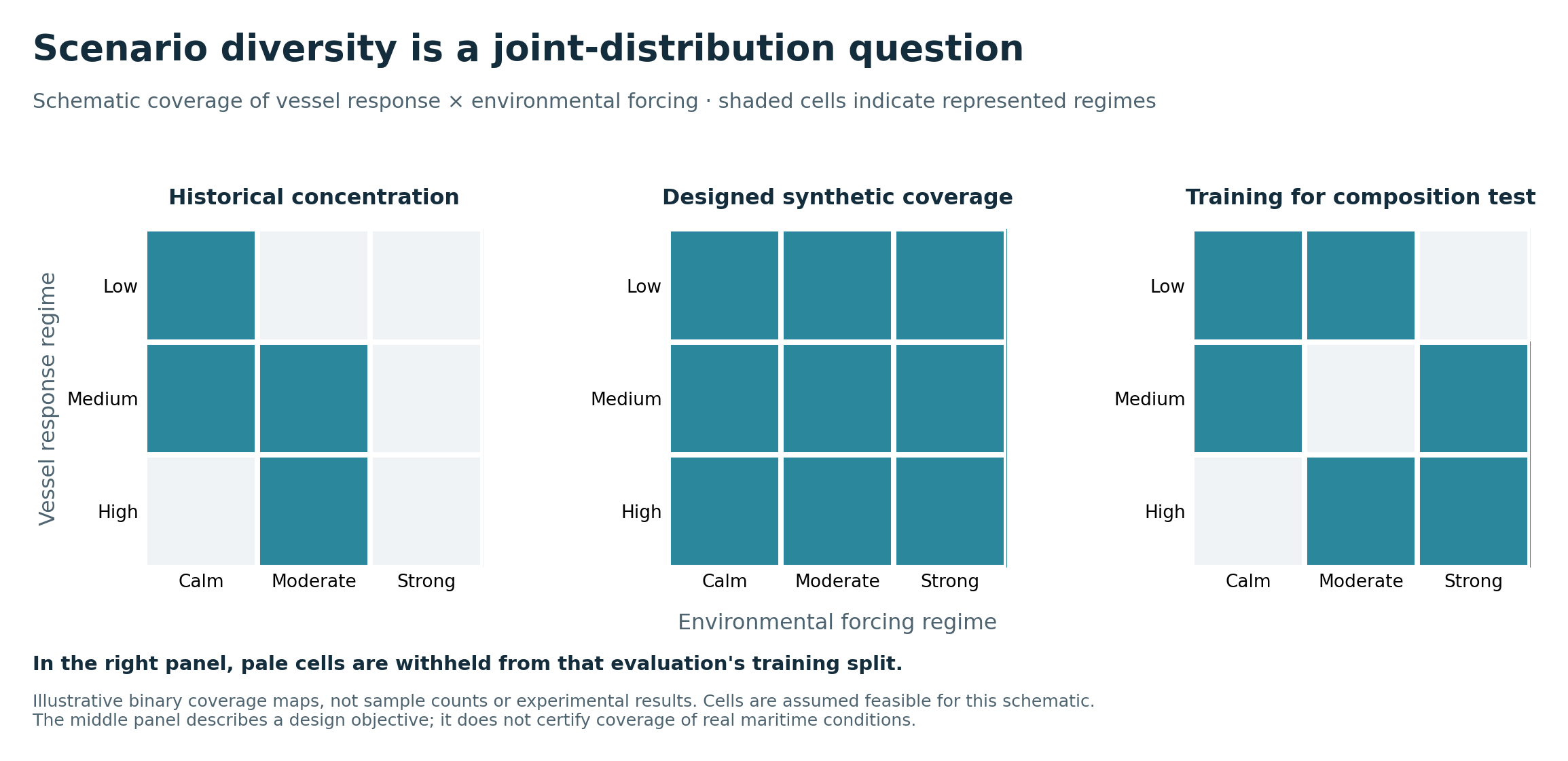
What “all possible compositions” should mean
Compositional coverage means deliberately representing a sufficiently broad, plausible set of combinations of vessel properties, operating conditions, forcing, and observation processes to support generalisation within a declared operating scope.
A useful aspiration for the scenario sampler is:
\[\operatorname{supp}(P_{\mathrm{target}}^{\mathrm{scenario}}) \subseteq \operatorname{supp}(Q_\phi).\]This design aspiration is not a necessary or sufficient condition for transfer, and it cannot be verified from AIS alone. A model may sometimes generalise beyond sampled support when learned structural regularities remain valid. Continuous variables cannot be exhausted by a finite dataset; some combinations are physically infeasible; and the simulator may omit real mechanisms. Moreover, nonzero sampling probability may be negligible. For a feasible scenario stratum \(C_j\) and \(n\) independent draws:
\[\mathbb{E}[N_j]=n\,Q_\phi(C_j).\]Thus, sampling weights, minimum per-stratum coverage, and explicit rare regime tests matter m. Crucially, withholding feasible combinations for evaluation tests something different from training on an expanded combination set whether representations generalise to compositions they were not explicitly shown.
5. Broad Simulation Does Not Remove the Simulation Gap
One pretraining strategy mixes real and synthetic observations in a shared representation:
\[P_\alpha^{\mathrm{obs}}=(1-\alpha)P_{\mathrm{real}}^{\mathrm{obs}} +\alpha P_{\mathrm{sim}}^{\mathrm{obs}},\qquad 0\leq\alpha\leq1.\]A model may learn to predict future records, reconstruct masked trajectory segments, or encode reusable windows. If simulator only latent labels are used for auxiliary supervision, that training signal must be identified separately; those labels do not suddenly become observed variables in real AIS.
Larger synthetic sets improve estimation under the chosen simulation distribution. They do not guarantee that the simulated vessel response, decision process, noise structure, or reporting regime matches deployment. Domain-adaptation theory, developed in part for classification settings, formalises the need for assumptions connecting source and target distributions (Ben-David et al., 2010). It motivates caution here rather than providing a direct guarantee for probabilistic AIS forecasting.
The practical test is therefore not “did pretraining loss improve?” but “did simulation-informed pretraining improve held-out real-data generalisation, calibration, and adaptation efficiency?” This must be compared against real-only pretraining, direct supervised baselines, and alternative simulation choices.
6. Broad Pretraining Needs Demonstrated Transfer
A reusable pretrained base should work across a declared family of downstream tasks, under transparent adaptation budgets. Let \(\theta_0\) denote pretrained parameters. For task \(\tau\), the adapted solution can be expressed as:
\[h_\tau=\mathcal{A}_\tau(\theta_0,D_\tau,c_\tau;B_\tau), \qquad \tau\in\mathcal{T}_{\mathrm{motion}}.\]Here \(D_\tau\) is labelled or otherwise usable task data, \(c_\tau\) is relevant task context, and \(B_\tau\) specifies the adaptation budget. Adaptation may use a frozen encoder, a shallow head, a parameter-efficient update, or fine-tuning. A trajectory forecasting decoder is not assumed to directly solve every task.
| Downstream task | Candidate reusable structure | Evidence needed |
|---|---|---|
| Probabilistic trajectory forecasting | Route modes and motion dynamics | Mode coverage, calibration, horizon-wise accuracy |
| Gap reconstruction | Temporal continuity and observation representations | Natural vs deliberately withheld gaps evaluated separately |
| Arrival-time prediction | Motion histories and route context | Defined arrival event; destination information where available |
| Anchorage / berth-state inference | Low-speed persistence and spatial context | Independent state labels, geographic transfer |
| Loitering / waiting classification | Temporal operating regimes | Separation from anchorage and drifting; independent labels |
| Congestion / queue modelling | Collective arrival and trajectory patterns | Port and temporal holdouts; interaction-aware baselines |
| Vessel interaction / rendezvous | Relative trajectories and context | Multi-vessel evidence; avoidance of identity shortcuts |
| Track-quality assessment | Expected reporting and motion consistency | Verified errors, not merely unusual movement |
| Activity / anomaly classification | Structured motion representations | Independent labels, false-positive control, shift robustness |
A stronger foundation claim combines broad pretraining with measurable adaptability across several meaningful tasks, vessels, seasons, regions, and observation regimes. This evaluation should hold adaptation data and compute budgets constant against capable task-specific baselines. The evaluation should separate vessel and voyage identities; hold out regions and time periods where relevant; introduce feasible unseen combinations; and report predictive error, distributional calibration, label efficiency, and failure modes.
Scope also matters, a maritime motion foundation is not automatically a foundation for deck imagery, machinery telemetry, intent attribution, compliance judgments, or all maritime applications as unusual motion alone does not establish intent or wrongdoing.
7. A Research Criterion for a Maritime Motion Foundation
The proposed framework implies three linked tests:
- Observation fidelity: Does the model handle the distinction between motion, measurement, irregular reports, and missingness without asserting unobserved physical variables as known?
- Coverage and generalisation: Does scenario design improve marginal, compositional, and dynamical representation, including feasible combinations withheld from training?
- Transfer efficiency: Does a shared pretrained base improve downstream tasks and data efficiency under controlled adaptation budgets relative to appropriate alternatives?
The first prevents a false causal claim, the second makes synthetic pretraining scientifically testable an the third tests whether the broadly pretrained base delivers the adaptability claimed of a foundation model.
References and Sources
- Bommasani, R., et al. (2021). On the Opportunities and Risks of Foundation Models. arXiv:2108.07258.
- US Coast Guard Navigation Center (n.d.). AIS Frequently Asked Questions and Class A AIS Position Reports. Reported vessel fields, reporting rates, and message structure.
- IALA (2016). Guideline 1082: An Overview of AIS. Reporting intervals for AIS station classes.
- Nguyen, D. and Fablet, R. (2024). TrAISformer: A Transformer Network with Sparse Augmented Data Representation and Cross Entropy Loss for AIS-based Vessel Trajectory Prediction. IEEE Access. DOI: 10.1109/ACCESS.2024.3349957. Original preprint: arXiv:2109.03958 (2021).
- Tobin, J., Fong, R., Ray, A., Schneider, J., Zaremba, W., and Abbeel, P. (2017). Domain Randomization for Transferring Deep Neural Networks from Simulation to the Real World. IROS / arXiv:1703.06907.
- Ben-David, S., Blitzer, J., Crammer, K., Kulesza, A., Pereira, F., and Vaughan, J. W. (2010). A theory of learning from different domains. Machine Learning, 79, 151–175.